How to Use VLOOKUP in Google Sheets? (Function, Examples)

Understanding the Google Sheets VLOOKUP Function

VLOOKUP is a powerful tool in Google Sheets that allows you to search for a specific value in a column of data and retrieve a corresponding value from another column. To make the most out of this function, it’s crucial to understand its inner workings. Let’s delve into the key aspects of the VLOOKUP function.

Google Sheets VLOOKUP Syntax

The syntax of VLOOKUP may seem intimidating at first glance, but breaking it down simplifies its understanding:

Google Sheets VLOOKUP Parameters

• search_key: This is the value you’re looking for in the first column of the specified range.
• range: This refers to the range of cells containing the data you want to search through. It’s crucial to select the correct range to ensure accurate results.
• index: This parameter denotes the column number in the selected range from which to return the corresponding value. The first column in the range is counted as 1, the second as 2, and so on.
• [is_sorted]: This is an optional parameter that indicates whether the first column in the range is sorted in ascending order. If set to TRUE or omitted, Google Sheets assumes that the data is sorted in ascending order, enabling it to perform a faster search using binary search. If set to FALSE, or 0, Google Sheets performs an exact match, which is useful for unsorted data.

Data Structure Requirements

For VLOOKUP to work effectively, your data must adhere to specific structural requirements:

• Table Format: Ensure your data is organized in a tabular format, with each column representing a different attribute or variable. VLOOKUP operates seamlessly within structured data tables.
• Consistent Data Types: Ensure consistency in data types, especially between the search key and the lookup column. Mixing data types can lead to errors or unexpected results.
• Unique Identifier: Ideally, your search key should be a unique identifier within the lookup column. This ensures that VLOOKUP returns the correct result without ambiguity.

Understanding these aspects of the VLOOKUP function will empower you to use it effectively in your Google Sheets projects, enhancing your data analysis capabilities.

How to Prepare Google Sheets Data for VLOOKUP?

Before diving into using the VLOOKUP function in Google Sheets, it’s essential to ensure that your data is properly structured and organized. Let’s explore the steps you need to take to prepare your data effectively.

Organizing Data Tables

Organizing your data into clear and structured tables is the first step in preparing for VLOOKUP. A well-organized table typically consists of rows and columns, with each column representing a different attribute or variable, and each row containing a specific data point or record. Ensure that your data tables have:

• Clear Headers: Use descriptive headers for each column to make it easy to understand the data.
• Consistent Formatting: Keep the formatting consistent across all cells in the table to avoid discrepancies in data interpretation.
• No Blank Rows or Columns: Remove any unnecessary blank rows or columns within the table to maintain clarity and avoid errors in VLOOKUP calculations.

By organizing your data tables effectively, you lay the foundation for accurate and efficient use of the VLOOKUP function.

Ensuring Data Compatibility

Data compatibility is crucial for the successful execution of VLOOKUP formulas. Here’s what you need to consider:

• Consistent Data Types: Ensure that the data types are consistent across the search key and lookup column. Mixing data types, such as numbers and text, can lead to errors or unexpected results.
• Text Case Sensitivity: Be mindful of text case sensitivity when using text values in your VLOOKUP formulas. Google Sheets treats uppercase and lowercase letters as different characters.
• Numeric Precision: Pay attention to numeric precision, especially when dealing with decimal values. Round off or format your data appropriately to ensure accurate VLOOKUP results.

Ensuring data compatibility sets the stage for seamless integration of the VLOOKUP function into your data analysis workflow.

Identifying Lookup and Reference Columns

Identifying the lookup column (where you’ll search for the value) and the reference column (from which you’ll retrieve the corresponding value) is essential for setting up your VLOOKUP formulas correctly. Consider the following:

• Selecting the Correct Lookup Column: Choose the column that contains the unique identifier or value you want to search for. This could be a product ID, customer name, or any other relevant identifier.
• Choosing the Reference Column: Determine which column contains the data you want to retrieve based on the search results. This could be the column containing prices, quantities, or any other related information.

By clearly identifying the lookup and reference columns, you ensure that your VLOOKUP formulas return accurate and meaningful results.

Preparing your data effectively lays the groundwork for successful utilization of the VLOOKUP function in Google Sheets. Taking the time to organize your data tables, ensure data compatibility, and identify the relevant columns will streamline your data analysis process and enhance the accuracy of your results.

How to Use VLOOKUP in Google Sheets?

Mastering the VLOOKUP function can greatly enhance your data analysis capabilities in Google Sheets. Let’s walk through each step of using VLOOKUP to search for and retrieve data efficiently.

1. Select Target Cell for VLOOKUP Formula

Next, select the cell where you want the result of your VLOOKUP formula to appear. This could be any cell within your spreadsheet where you want the retrieved data to be displayed.

2. Enter the VLOOKUP Formula

Now it’s time to enter the VLOOKUP formula into the selected cell. The basic structure of the formula is as follows:

3. Specify Lookup Value

Replace search_key in the formula with the value you want to search for. This could be a specific text string, number, date, or even a reference to another cell containing the value.

4. Choose the Range to Search

Replace range with the range of cells that contains the data you want to search through. This range typically includes both the lookup column (where the search will be conducted) and the reference column (from which data will be retrieved).

5. Designate Column Index

Specify index as the column number within the range from which you want to retrieve the corresponding value. Count the columns starting from 1, with the first column in the range being 1, the second column being 2, and so on.

6. Define Exact or Approximate Match

Optionally, specify whether you want an exact or approximate match by including TRUE or FALSE for the [is_sorted] parameter. If omitted or set to TRUE, Google Sheets assumes the data is sorted in ascending order and performs an approximate match. If set to FALSE, Google Sheets performs an exact match.

7. Handle Errors

Finally, it’s essential to handle any potential errors that may arise when using the VLOOKUP function. Common errors include #N/A, which indicates that the search key was not found in the lookup column. You can use the IFERROR function to display a custom message or value instead of the error.

By following these step-by-step instructions, you can effectively utilize the VLOOKUP function in Google Sheets to search for and retrieve data with precision and accuracy. Experiment with different scenarios and data sets to become proficient in using VLOOKUP for your data analysis needs.

Practical Examples of VLOOKUP Usage

Now that you’ve learned the fundamentals of the VLOOKUP function, let’s explore some practical examples to illustrate its versatility and usefulness in real-world scenarios.

Basic VLOOKUP for Simple Data Retrieval

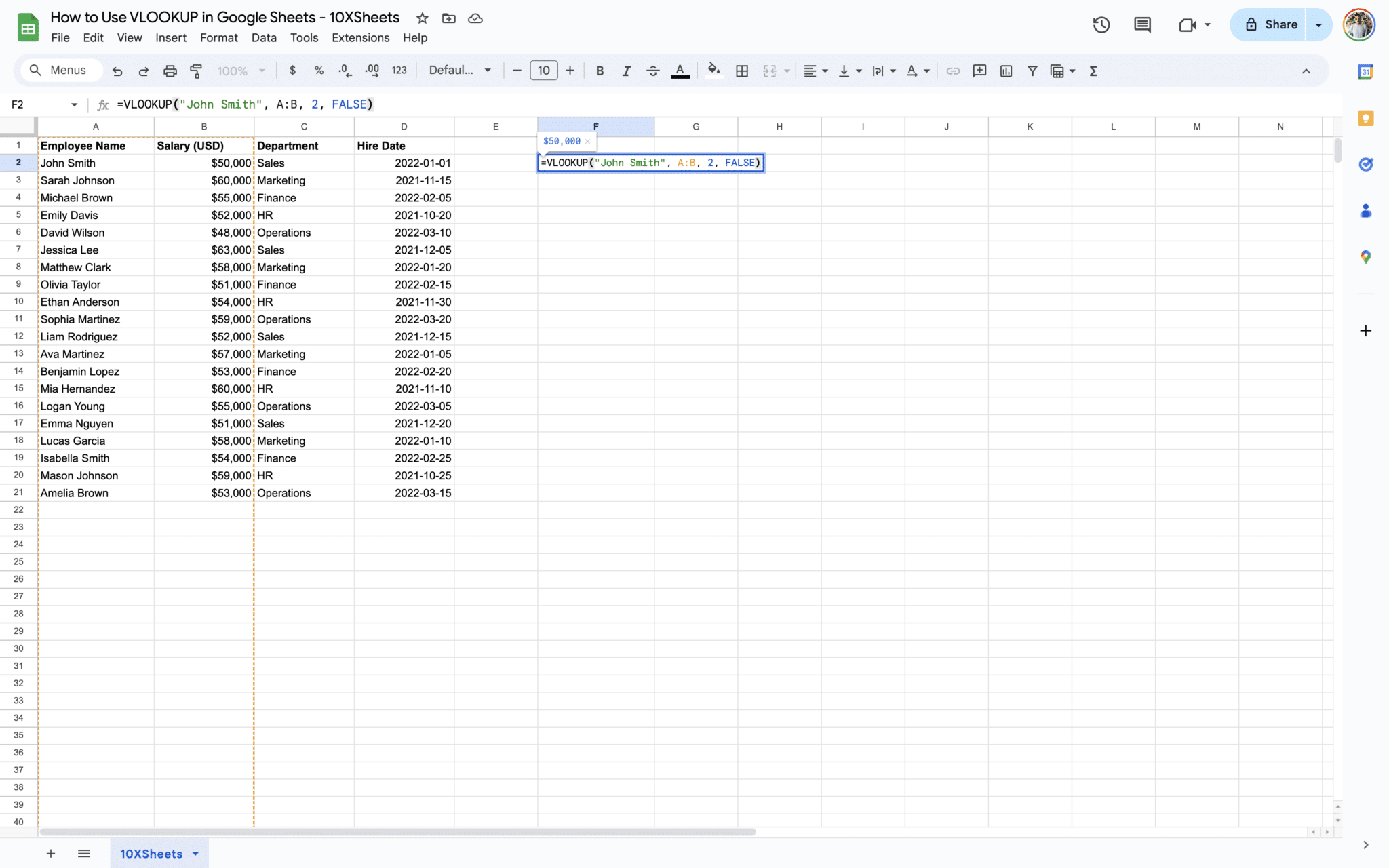
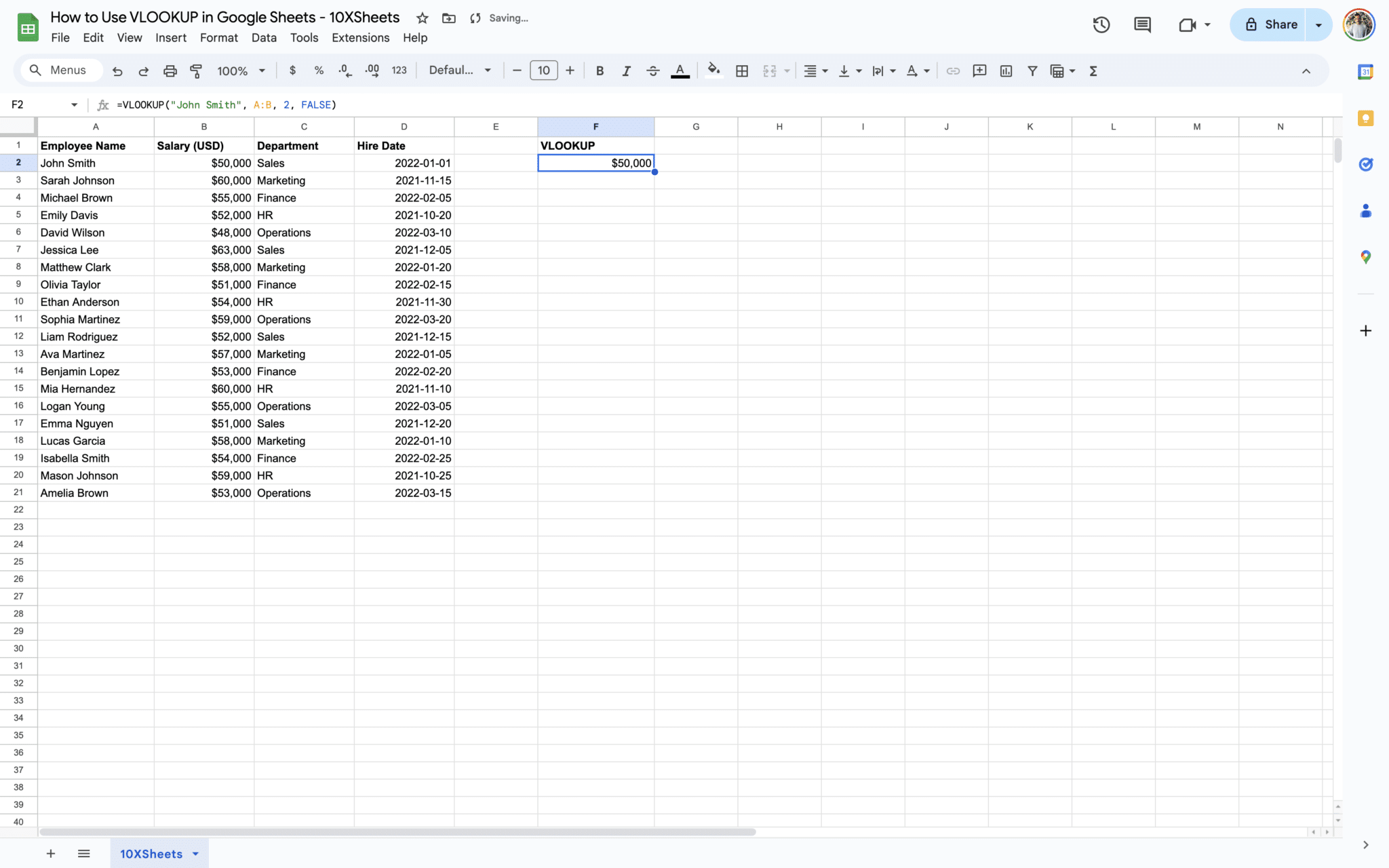
One of the most common use cases for VLOOKUP is simple data retrieval. Suppose you have a table with employee names in column A and their corresponding salaries in column B. You can use VLOOKUP to quickly retrieve the salary of a specific employee based on their name.

For example:

This formula searches for “John Smith” in column A and returns the corresponding salary from column B.

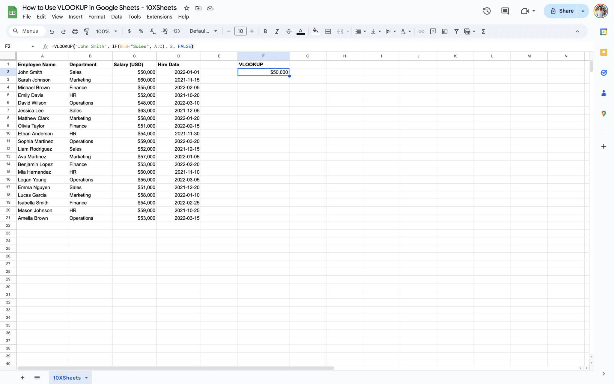
VLOOKUP with Multiple Criteria

Sometimes, you may need to perform a VLOOKUP based on multiple criteria. In such cases, you can combine VLOOKUP with other functions such as IF and AND to create more complex search criteria.

Suppose you have a table with employee names in column A, their departments in column B, and their salaries in column C. You want to find the salary of an employee named “John Smith” who works in the “Sales” department.

You can use the following formula:

This formula searches for the value “John Smith” in column A and checks if the corresponding value in column B is “Sales” using the IF function. If the condition is met, it returns the corresponding value from column C using VLOOKUP.

VLOOKUP for Dynamic Data Updates

VLOOKUP can also be used for dynamic data updates. Suppose you have a table that is regularly updated with new information. By using named ranges in your VLOOKUP formulas, you can ensure that your formulas automatically update when new data is added.

For example:

In this formula, “Employee_Data” is a named range that refers to the range of cells containing employee data. As new data is added to the table, the named range automatically adjusts, ensuring that your VLOOKUP formula remains accurate and up-to-date.

Advanced VLOOKUP Scenarios

VLOOKUP can be used in more advanced scenarios, such as retrieving data from multiple sheets or workbooks, or performing nested VLOOKUP functions. These advanced techniques allow you to handle complex data analysis tasks with ease.

For example:

In this formula, $B$1 refers to a cell containing the name of the sheet from which you want to retrieve data. By combining INDIRECT with VLOOKUP, you can dynamically reference different sheets based on user input.

By exploring these practical examples, you can gain a deeper understanding of how to leverage the power of the VLOOKUP function in various data analysis scenarios. Experiment with different formulas and datasets to become proficient in using VLOOKUP for your specific needs.

Google Sheets VLOOKUP Tips and Best Practices

To maximize the effectiveness of your VLOOKUP usage and streamline your workflow, consider implementing the following tips and best practices.

Using Named Ranges for Clarity

Named ranges provide a convenient way to refer to specific ranges of cells in your spreadsheet. By assigning meaningful names to ranges, you can make your formulas more readable and easier to understand.

For example, instead of using A1:B10 to refer to a range containing employee data, you could name the range “Employee_Data.” Then, your VLOOKUP formula would look like this:

Utilizing Absolute and Relative Cell References

Understanding when to use absolute and relative cell references in your VLOOKUP formulas is crucial for their accuracy and flexibility.

• Absolute References: Use absolute references (e.g., $A$1) when you want a cell reference to remain constant, even when the formula is copied to other cells. Absolute references are useful for referencing fixed values, such as lookup tables or constants.
• Relative References: Use relative references (e.g., A1) when you want the cell reference to adjust relative to the formula’s location when copied to other cells. Relative references are helpful for referencing data that is arranged in a consistent manner across rows or columns.

Employing VLOOKUP with Other Functions

VLOOKUP can be combined with other functions in Google Sheets to perform more complex calculations and data manipulations. Here are a few examples:

• IF Function: Use the IF function to handle situations where the search key may not exist in the lookup column. You can customize the output based on whether the search key is found or not.
• INDEX and MATCH Functions: Instead of using VLOOKUP, consider using the INDEX and MATCH functions together. This combination offers more flexibility and can handle situations where the lookup column is not the first column in the range.

Troubleshooting Common Errors

Even with careful preparation, errors can occur when using VLOOKUP. Here are some common errors and how to troubleshoot them:

• #N/A Error: This error occurs when the search key is not found in the lookup column. Double-check the search key and ensure that it exists in the lookup column. You can use the IFERROR function to handle this error gracefully.
• Incorrect Results: If you’re getting incorrect results, check the data types of the search key and the values in the lookup column. Make sure they match or convert them if necessary.
• Sorted Data Requirement: If you’re using approximate matching with VLOOKUP, ensure that your data is sorted in ascending order. If not, switch to exact matching by setting the [is_sorted] parameter to FALSE.

By implementing these tips and best practices, you can enhance your proficiency in using the VLOOKUP function and avoid common pitfalls. Experiment with different scenarios and formulas to gain confidence in your data analysis skills.