Built for Google Sheets
Your next model—without the cold start
Open a workbook with clear tabs, labeled drivers, and layouts you can reshape in minutes—forecasting, P&L, cohorts, and more. Spend energy on the decision, not rebuilding the grid.
Find your template
How to Use SUMIF in Google Sheets (With Multiple Criteria)
Ever wondered how to efficiently analyze data in Google Sheets, effortlessly summing values based on specific conditions? If you've found yourself grappling with this challenge, then mastering the SUMIF function is the key. In this guide, we'll explore everything you need to know about leveraging SUMIF in Google Sheets. From understanding its syntax and parameters to diving into practical applications and advanced techniques, you'll discover how to wield SUMIF effectively for data analysis, expense tracking, budgeting, and more.
What is the SUMIF Function in Google Sheets?
The SUMIF function in Google Sheets is a powerful tool that allows you to perform conditional summations based on specific criteria. It simplifies the process of summarizing data by summing only the values that meet certain conditions, thereby providing valuable insights into your dataset. Understanding how to use SUMIF effectively can significantly enhance your ability to analyze and manipulate data within Google Sheets.
Importance of Using SUMIF in Google Sheets
-
Efficiency: SUMIF streamlines the process of calculating sums based on specific conditions, saving you time and effort compared to manual calculations.
-
Flexibility: With SUMIF, you can easily adapt your calculations to different scenarios by adjusting the criteria as needed, without altering the underlying structure of your spreadsheet.
-
Accuracy: By automating the summation process, SUMIF reduces the risk of human error that may occur with manual calculations, ensuring greater accuracy in your results.
-
Insightful Analysis: SUMIF enables you to perform detailed analyses of your data, allowing you to uncover patterns, trends, and outliers that may not be immediately apparent through manual examination.
-
Decision Making: The insights gained from SUMIF calculations can inform important decision-making processes, whether in business, finance, project management, or personal budgeting.
In summary, the SUMIF function is an indispensable tool for anyone working with data in Google Sheets. Its efficiency, flexibility, accuracy, and ability to provide insightful analysis make it a valuable asset for a wide range of applications. Whether you're a novice spreadsheet user or an experienced data analyst, mastering SUMIF can greatly enhance your productivity and effectiveness in Google Sheets.
Understanding SUMIF Function
The SUMIF function in Google Sheets is a fundamental tool for performing conditional summation operations. It allows you to sum values based on specific conditions or criteria. Let's delve deeper into the intricacies of how SUMIF works and explore its syntax, parameters, and practical examples.
Syntax of SUMIF
The syntax of the SUMIF function follows a simple pattern:
=SUMIF(range, criteria, [sum_range])
Parameters of SUMIF
Here's what each part of the syntax represents:
-
range: The range parameter is the set of cells that you want Google Sheets to evaluate against your criteria. It's where the function will look for the values that meet the specified condition.
-
criteria: The criteria parameter is the condition or criterion that determines which cells should be included in the sum. It can be a number, text, expression, or reference to another cell.
-
sum_range: The sum_range parameter is optional. It allows you to specify the range of cells containing the values that you want to sum. If omitted, SUMIF will use the same range specified in the range parameter for both evaluation and summation.
Examples illustrating SUMIF function usage
Let's consider a few examples to better understand how to use the SUMIF function in practical scenarios:
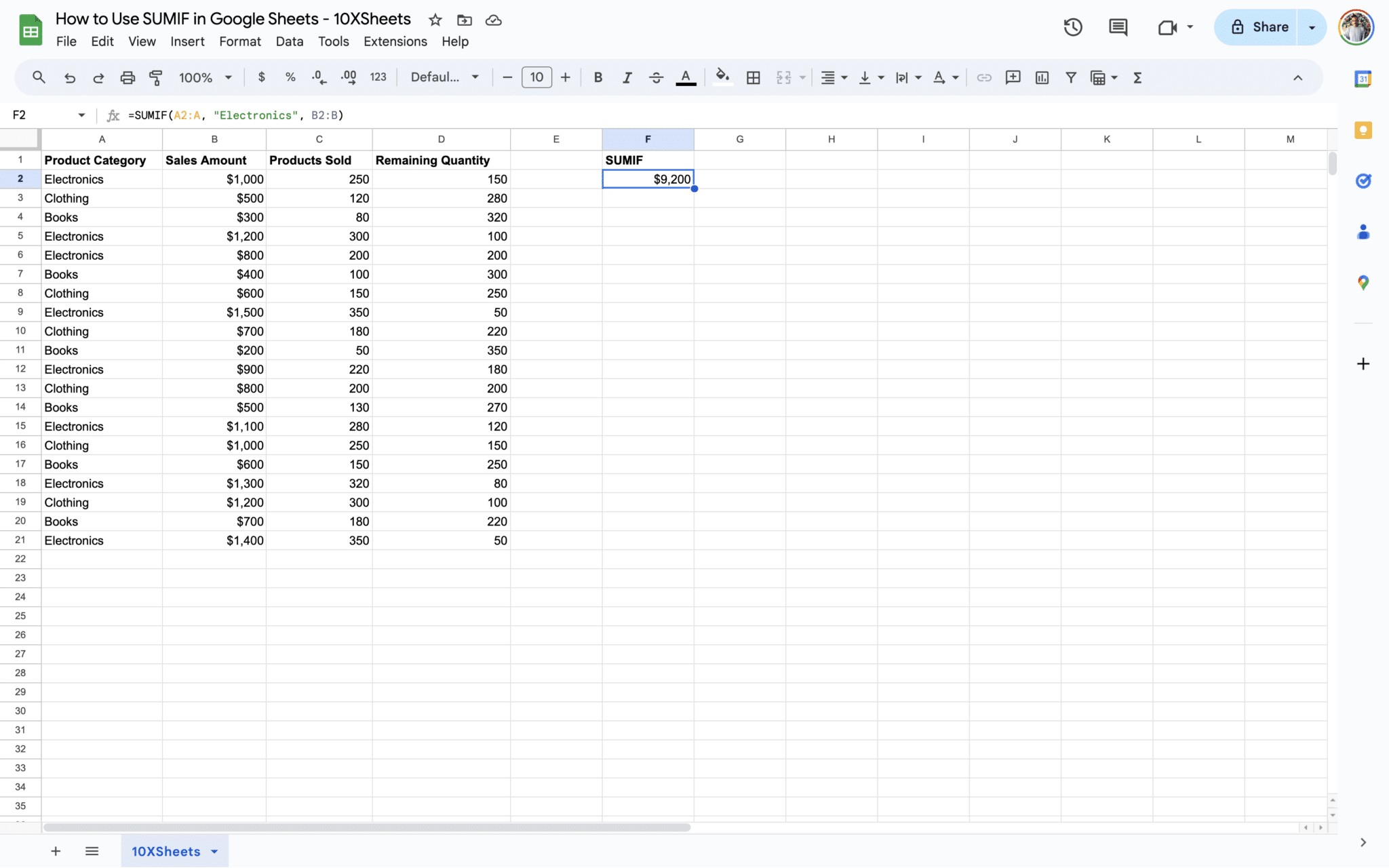
- Example 1: Summing Sales Amounts Based on Product Categories
=SUMIF(A2:A, "Electronics", B2:B)
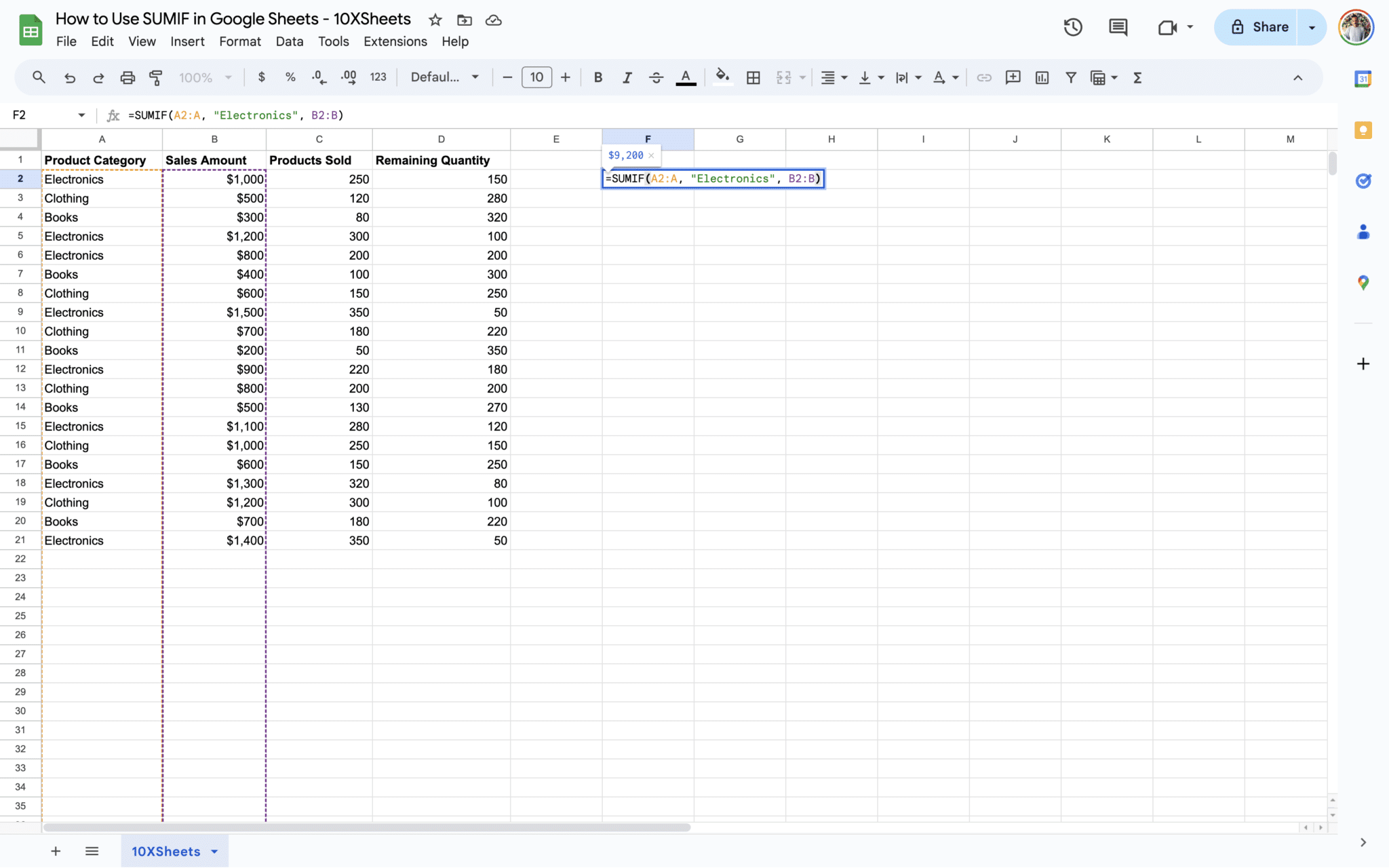
This formula sums all sales amounts in column B starting from B2 where the corresponding product category in the range A2:A is "Electronics".
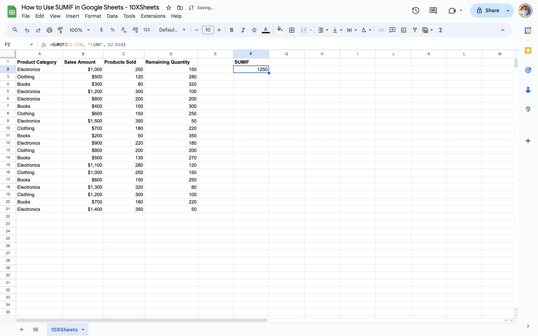
- Example 2: Conditional Summation Based on Numeric Criteria
=SUMIF(C2:C10, ">100", D2:D10)
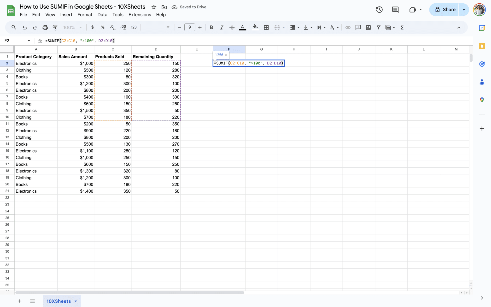
Here, the formula sums all values from the range D2:D10 where the corresponding value in the range C2:C10 is greater than 100.
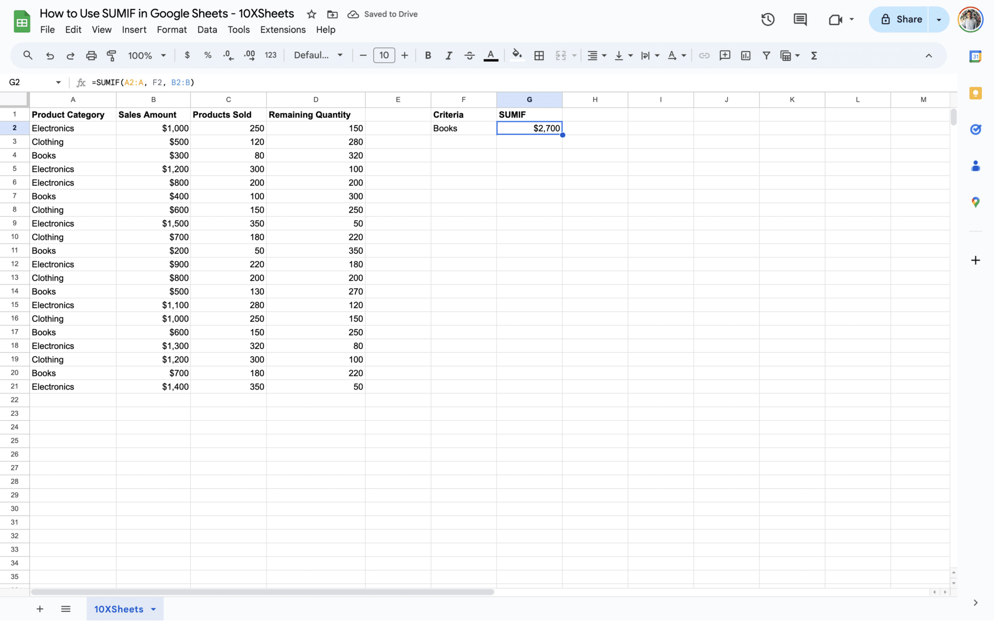
- Example 3: Dynamic Summation Using Cell References
=SUMIF(A2:A, F2, B2:B)
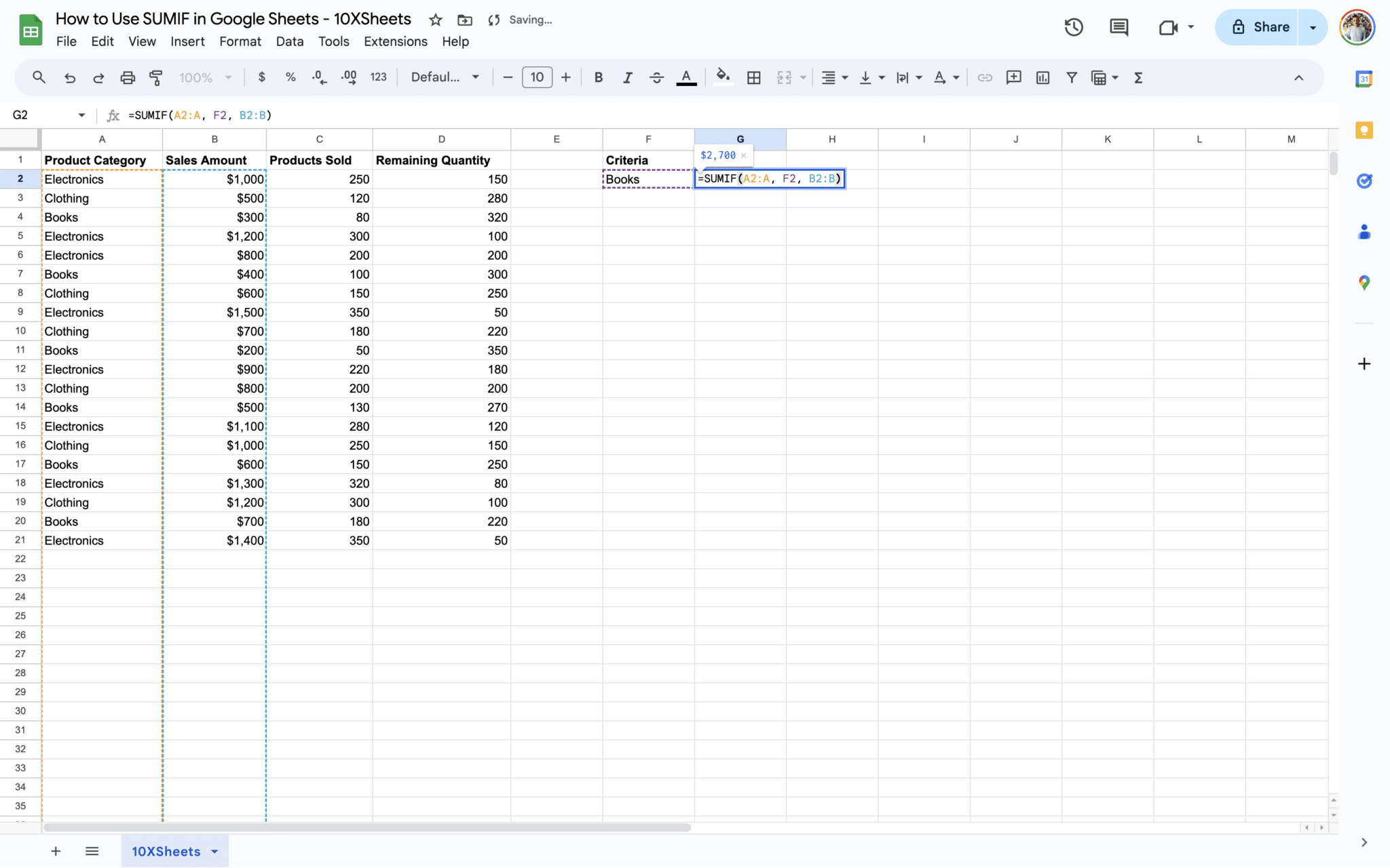
In this formula, the criteria for summation is taken from cell F2. It sums all values from the range B2:B where the corresponding value in the range A2:A matches the value in cell F2.
These examples demonstrate the versatility of the SUMIF function and how it can be customized to meet specific requirements in your Google Sheets projects.
How to Use SUMIF in Google Sheets?
Let's explore some fundamental ways to apply the SUMIF function for simple calculations and how you can utilize cell references to enhance the flexibility of your formulas.
Applying SUMIF for Simple Calculations
One of the most common use cases for SUMIF is to perform straightforward summations based on specific criteria. This could involve summing values that meet a certain condition or criterion within a dataset.
For instance, suppose you have a list of expenses in one column and corresponding categories in another. You might want to sum all expenses in the "Utilities" category. Here's how you can do it:
=SUMIF(B2:B10, "Utilities", A2:A10)
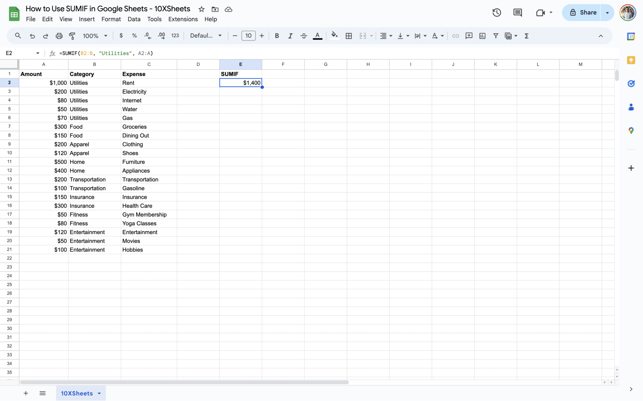
In this example:
-
B2:B10 represents the range containing categories.
-
"Utilities" is the criterion or condition we're looking for.
-
A2:A10 is the range containing the expenses to be summed.
The SUMIF function identifies all cells in the range B2:B10 that contain "Utilities" and then sums the corresponding expenses from A2:A10.
Utilizing Cell References in SUMIF Formulas
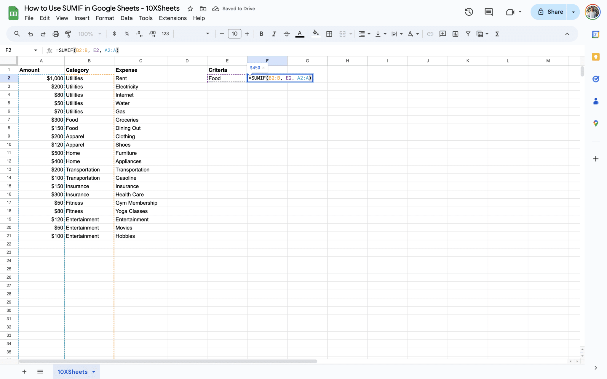
To make your SUMIF formulas more dynamic and adaptable, you can use cell references for criteria instead of hardcoding values directly into the formula. This allows you to change the criteria without modifying the formula itself.
For example, let's say you have a cell (E2) where you input the category you want to sum. Your SUMIF formula would then look like this:
=SUMIF(B2:B, E2, A2:A)
In this formula:
-
B2:B is still the range containing categories.
-
E2 now holds the criterion dynamically.
-
A2:A remains the range containing the values to be summed.
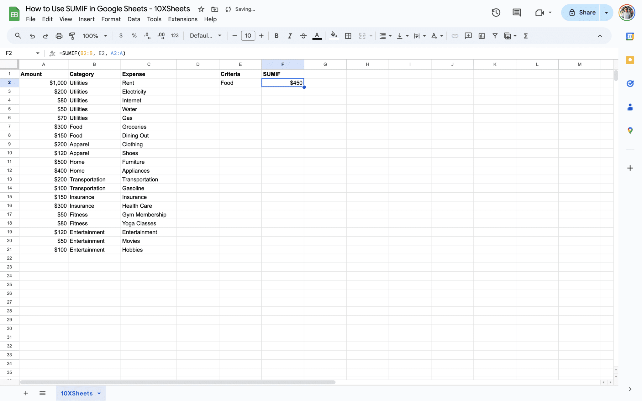
By changing the value in cell E2, you can instantly update the criteria for your SUMIF calculation without having to edit the formula directly. This approach offers greater flexibility and ease of use, especially when dealing with changing datasets or scenarios.
Advanced Techniques with SUMIF in Google Sheets
Now, let's delve into some advanced techniques that leverage the flexibility and power of the SUMIF function. These techniques allow you to perform more complex calculations and handle diverse scenarios within your Google Sheets projects.
Nesting SUMIF with Other Functions
One of the most powerful capabilities of Google Sheets is its ability to nest functions within each other. By combining SUMIF with other functions, you can create sophisticated formulas to meet your specific requirements.
For example, suppose you have a dataset containing sales data for multiple products and regions. You want to calculate the total sales for a particular product in a specific region. You can achieve this by nesting SUMIF within another function like IF or INDEX/MATCH.
-
A2:A100 represents the range containing regions.
-
B2:B100 contains the product names.
-
C2:C100 holds the criteria for the product "Product_A".
-
D2:D100 contains the sales data to be summed.
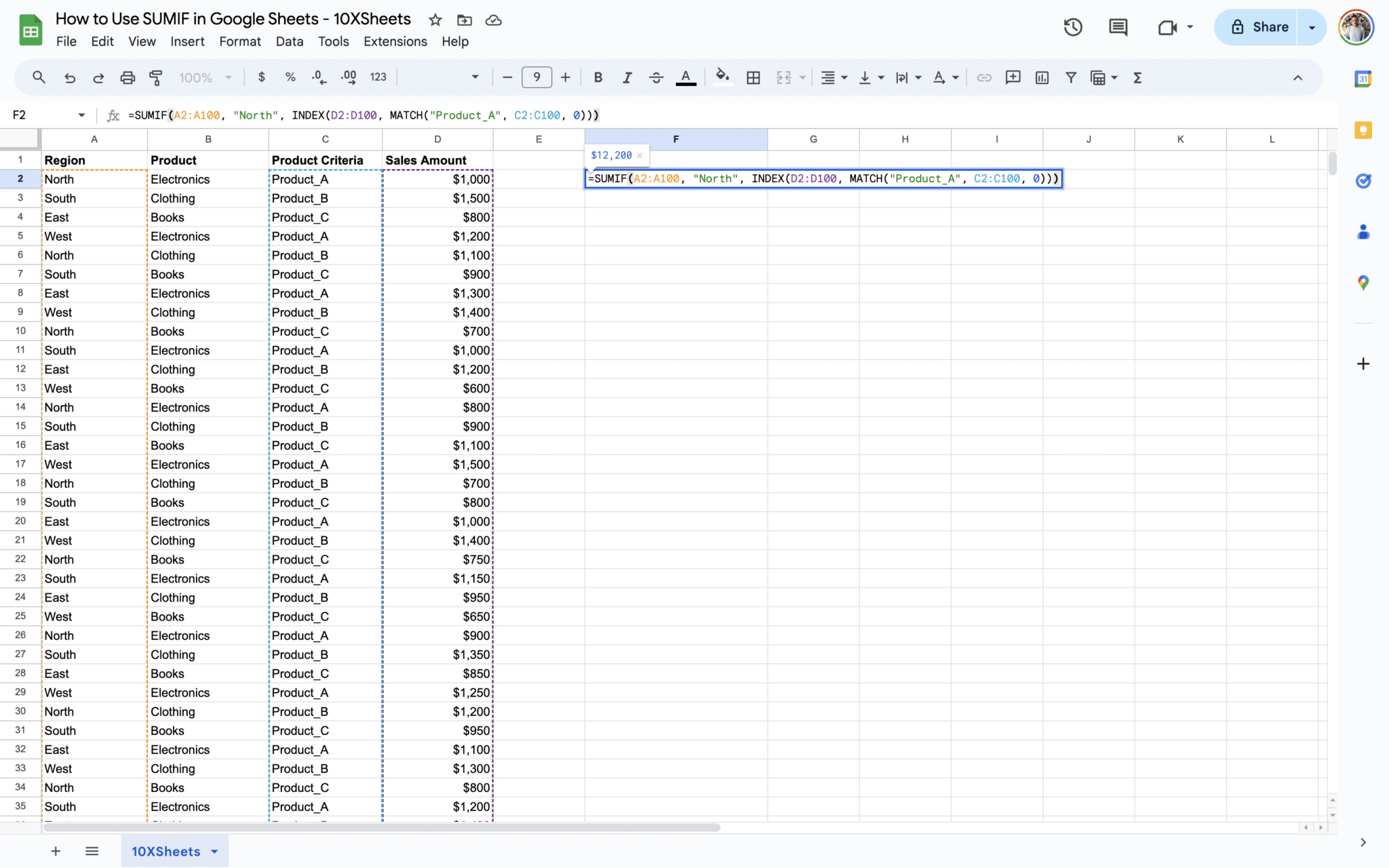
Here's a hypothetical scenario where you use SUMIF nested within INDEX/MATCH to calculate total sales for the product "Product_A" in the region "Region_X":
=SUMIF(A2:A100, "North", INDEX(D2:D100, MATCH("Product_A", C2:C100, 0)))
-
SUMIF(A2:A100, "North", …): This part of the formula sums the sales amounts from column D where the corresponding region in column A is "North".
-
INDEX(D2:D100, MATCH("Product_A", C2:C100, 0)): This part of the formula retrieves the sales data from column D where the corresponding product criteria in column C is "Product_A". The MATCH function searches for the position of "Product_A" within the range C2:C100, and INDEX returns the corresponding sales amount from column D based on the position found by MATCH.
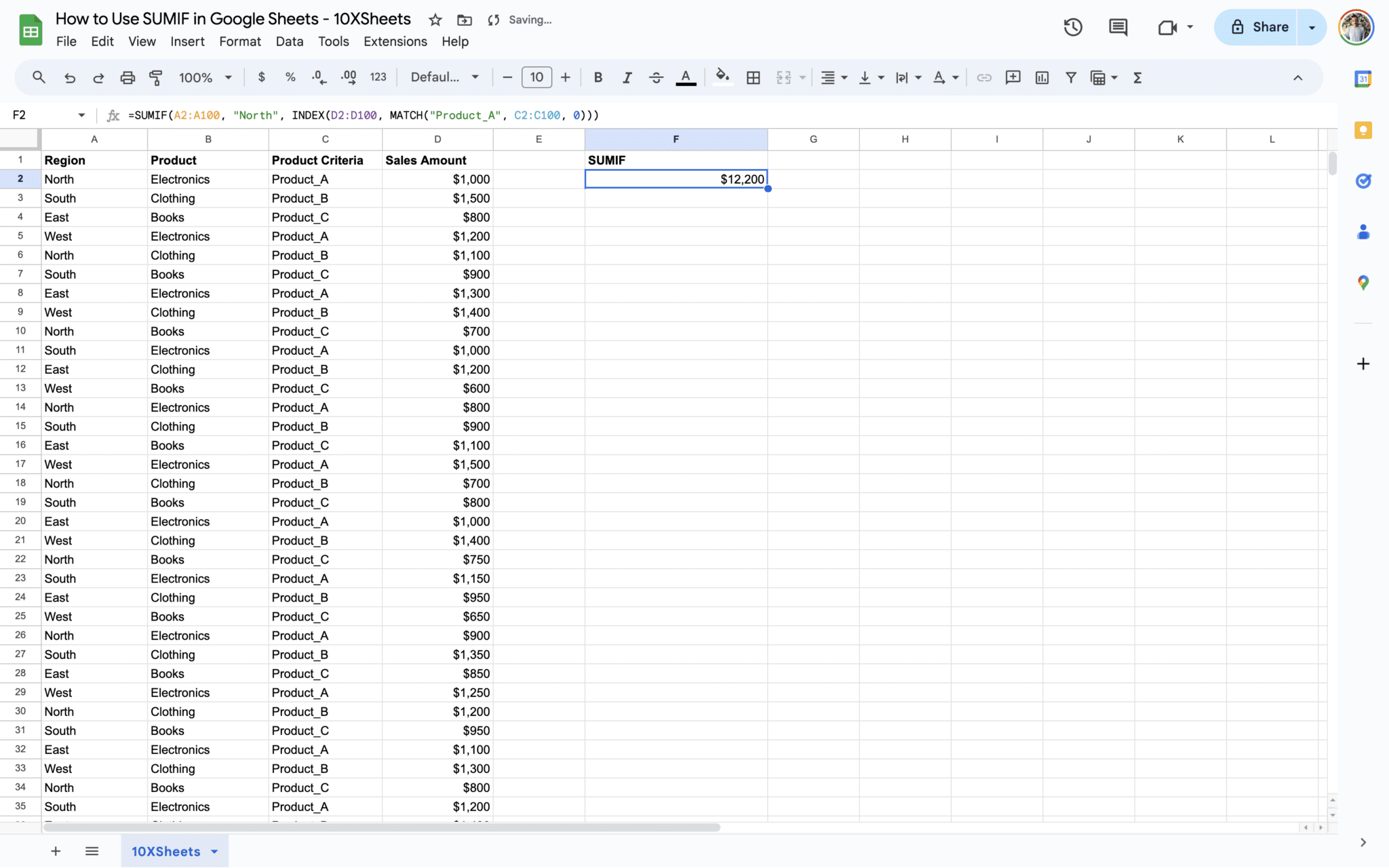
By nesting SUMIF within INDEX/MATCH, you can dynamically retrieve the sales data for the specified product and region.
Incorporating Logical Operators in SUMIF
Another advanced technique involves using logical operators within the criteria of the SUMIF function. This allows you to create more flexible conditions for summation, such as greater than, less than, equal to, etc.
For instance, let's say you want to sum all sales amounts that fall within a certain range. You can use logical operators like ">" and " =SUMIF(C2:C, ">250", B2:B)
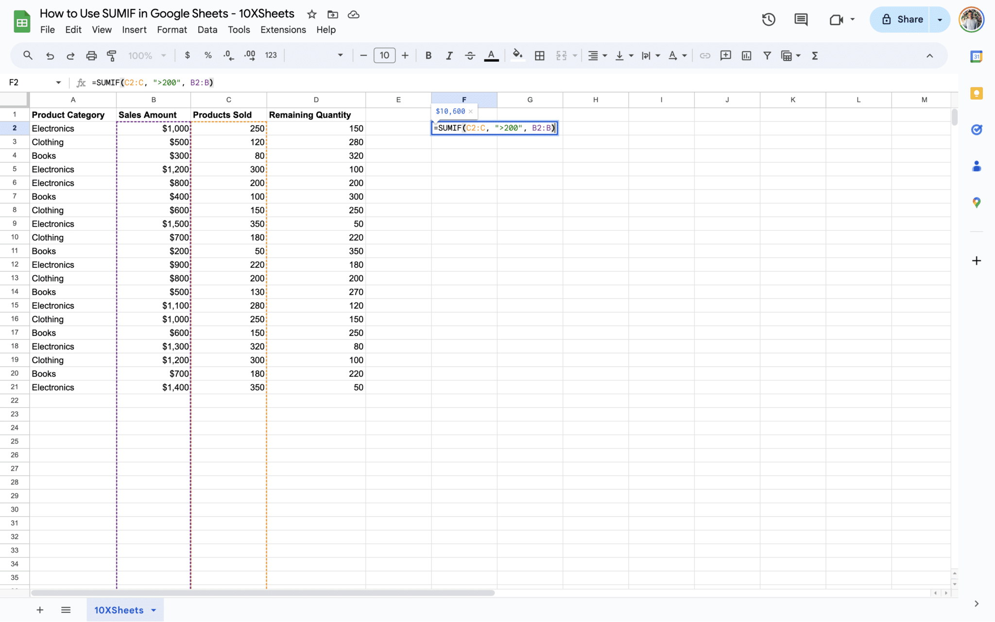
In this formula, SUMIF sums all values in the range B2:B where the corresponding values in the range C2:C are greater than 250. This technique enables you to perform complex calculations based on specific conditions.

Using Wildcards in SUMIF Criteria
Wildcards are special characters that represent unknown or variable characters. In SUMIF criteria, you can use wildcards like asterisk (*) and question mark (?) to match patterns within your data.
For instance, suppose you want to sum all sales amounts for products that start with the letter "A". You can use the asterisk wildcard (*) to match any characters following "A". Here's how:
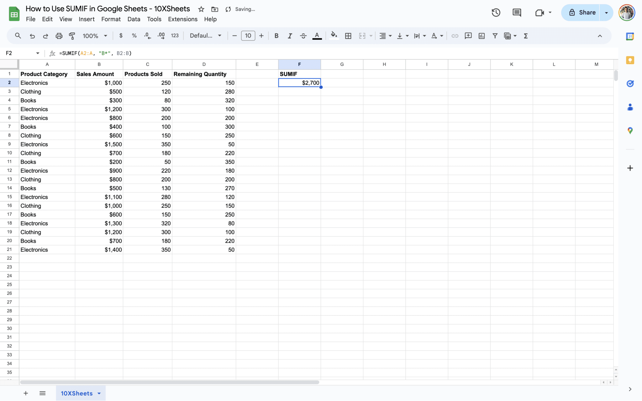
=SUMIF(A2:A, "B*", B2:B)
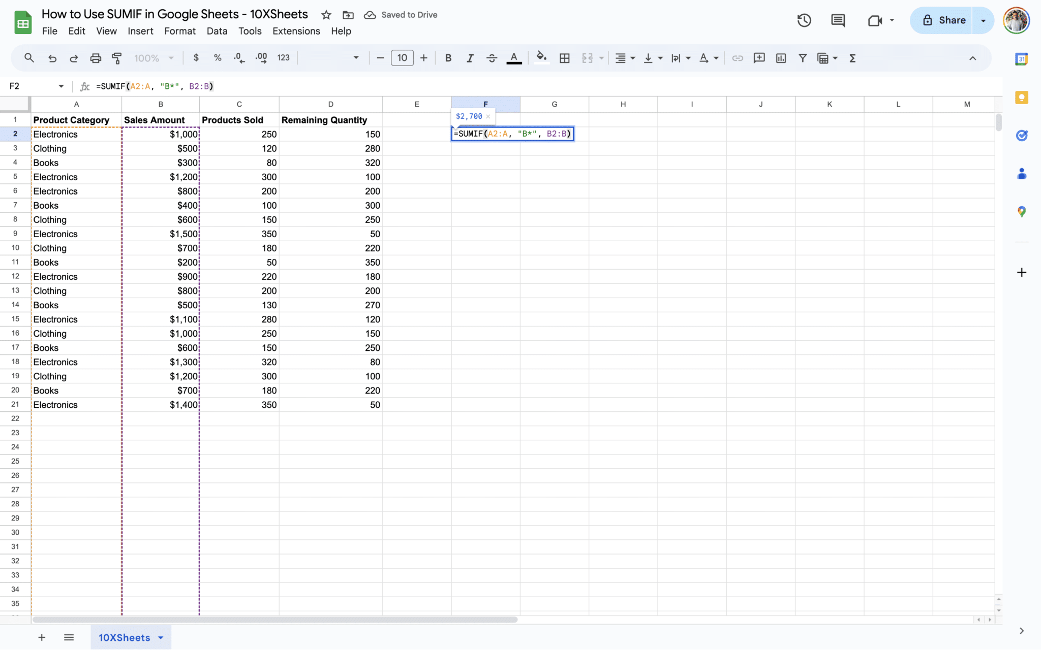
In this formula, SUMIF sums all values in the range B2:B where the corresponding values in the range A2:A start with the letter "B" (e.g., Books).
By incorporating wildcards into your SUMIF criteria, you can perform pattern matching and extract relevant data from your dataset more effectively.
Practical Applications of SUMIF
Now, let's explore some real-world scenarios where you can apply the SUMIF function to analyze data, track expenses, and manage budgets effectively within your Google Sheets projects.
Analyzing Sales Data with SUMIF
One of the most common applications of SUMIF is in analyzing sales data. Whether you're managing a business or studying market trends, SUMIF can help you extract valuable insights from your sales data.
For example, suppose you have a spreadsheet containing sales transactions with product categories, sales amounts, and dates. You can use SUMIF to calculate total sales for specific product categories or time periods.
Let's say you want to analyze the total sales for the "Electronics" category. You can use a SUMIF formula like this:
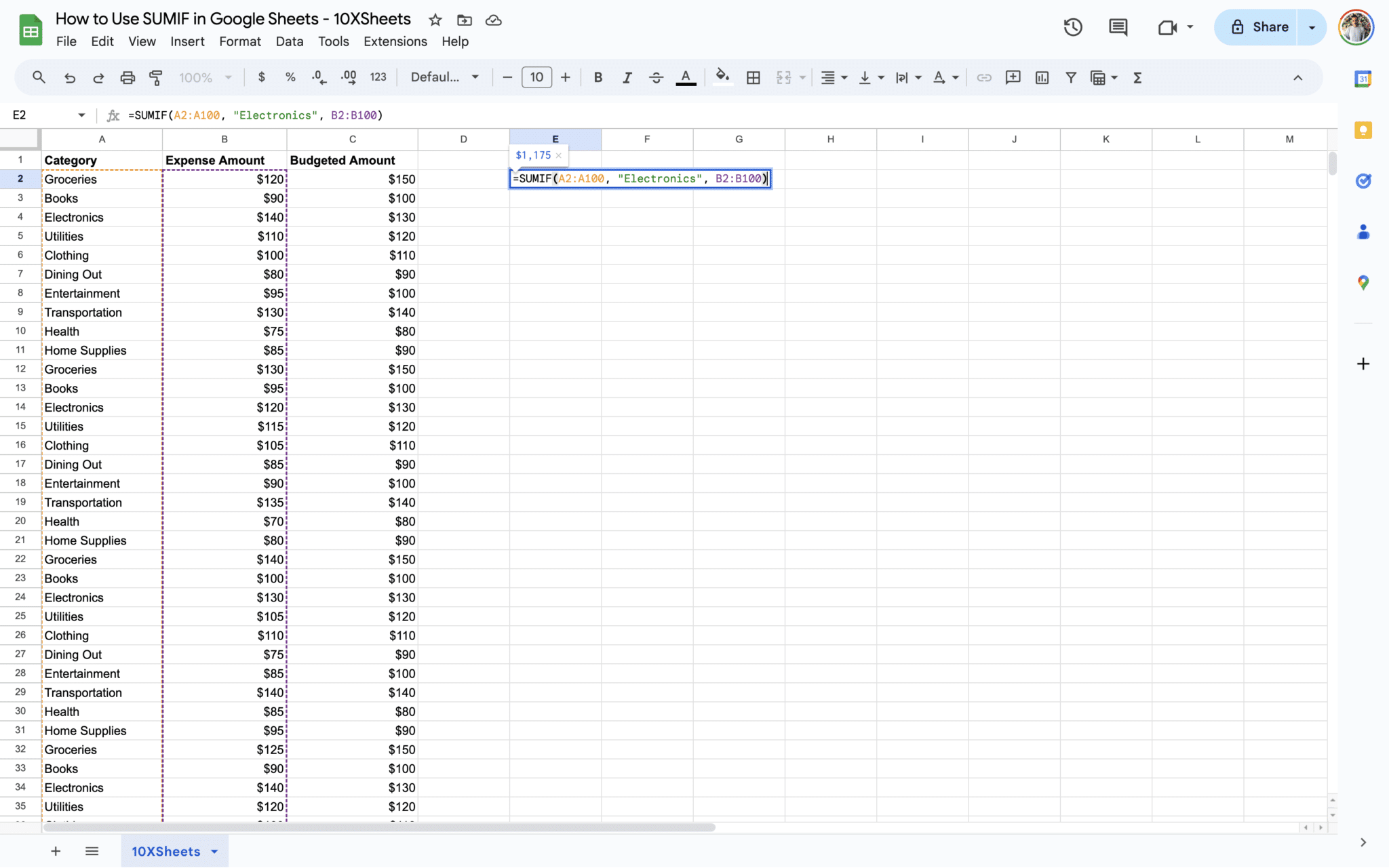
=SUMIF(A2:A100, "Electronics", B2:B100)
In this formula:
-
A2:A100 represents the range containing product categories.
-
"Electronics" is the criterion for the "Electronics" category.
-
B2:B100 contains the corresponding sales amounts to be summed.
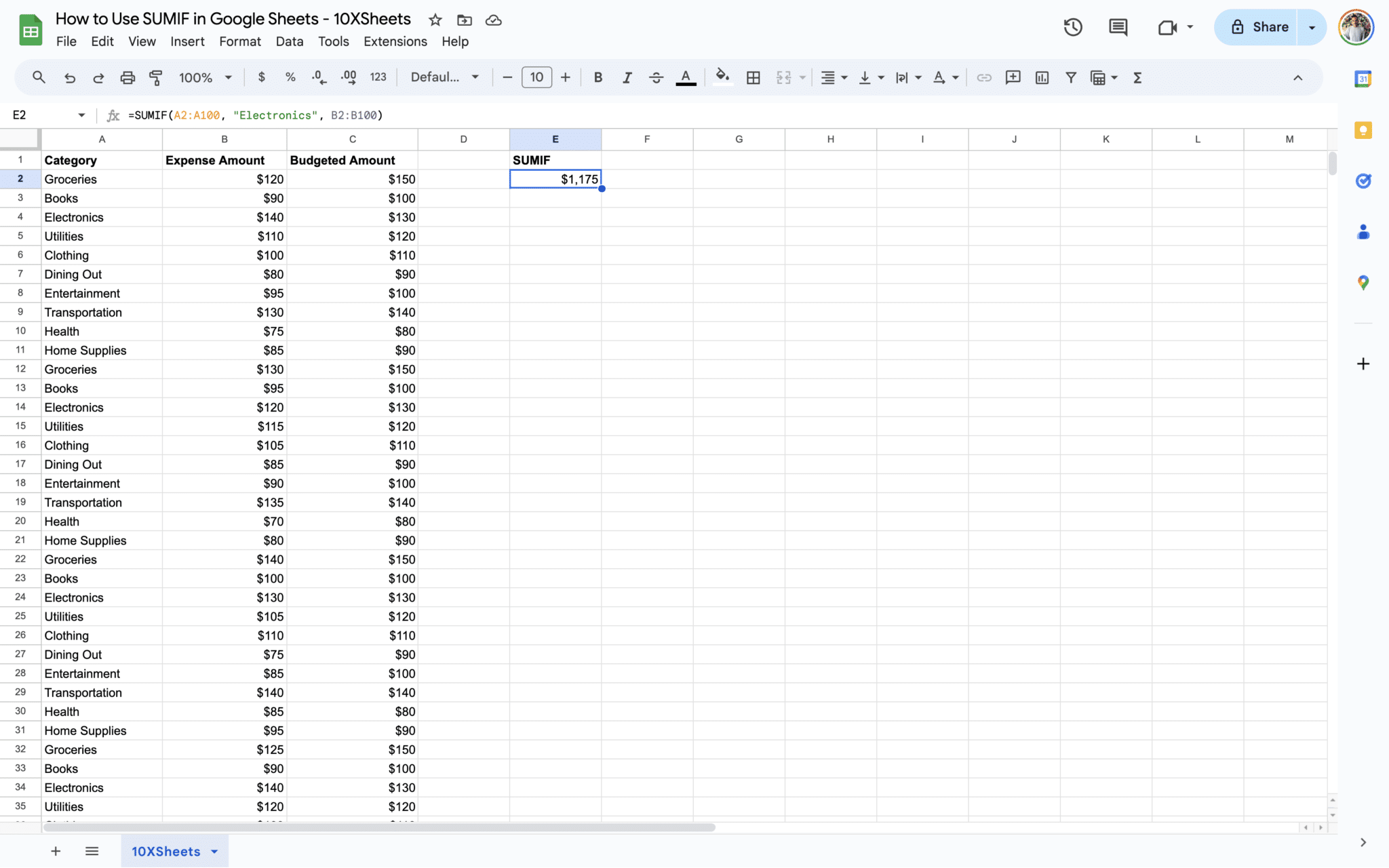
By applying SUMIF to your sales data, you can gain insights into which product categories are performing well and identify areas for improvement.
Tracking Expenses Using SUMIF
Another practical application of SUMIF is in tracking expenses, whether for personal budgeting or business expense management. SUMIF allows you to categorize and sum expenses based on specific criteria, making it easier to monitor your spending habits.
For instance, suppose you maintain a spreadsheet to track your monthly expenses, including categories like groceries, utilities, and entertainment. You can use SUMIF to calculate total expenses for each category.
Here's an example of how you can track your grocery expenses:
=SUMIF(A2:A100, "Groceries", B2:B100)
![]()
In this formula:
-
A2:A100 represents the range containing expense categories.
-
"Groceries" is the criterion for the grocery category.
-
B2:B100 contains the corresponding expense amounts to be summed.
![]()
By regularly updating and analyzing your expense tracking spreadsheet with SUMIF, you can gain valuable insights into your spending patterns and make informed decisions to manage your finances better.
Conditional Budgeting with SUMIF
Lastly, SUMIF can be a powerful tool for conditional budgeting, allowing you to set specific criteria for budget categories and track your expenses accordingly. This enables you to monitor your spending and stay within your budget limits effectively.
For example, let's say you have a monthly budget spreadsheet with budget categories such as groceries, transportation, and entertainment. You can use SUMIF to compare your actual expenses against your budget targets for each category.
Here's how you can calculate the variance between actual expenses and budgeted amounts for groceries:
=SUMIF(A2:A100, "Groceries", B2:B100) - SUMIF(A2:A100, "Groceries", C2:C100)
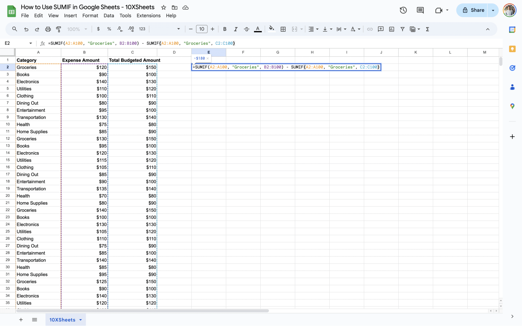
In this formula:
-
A2:A100 represents the range containing budget categories.
-
"Groceries" is the criterion for the grocery category.
-
B2:B contains the actual expense amounts to be summed.
-
C2:C2 contains the budgeted amounts.
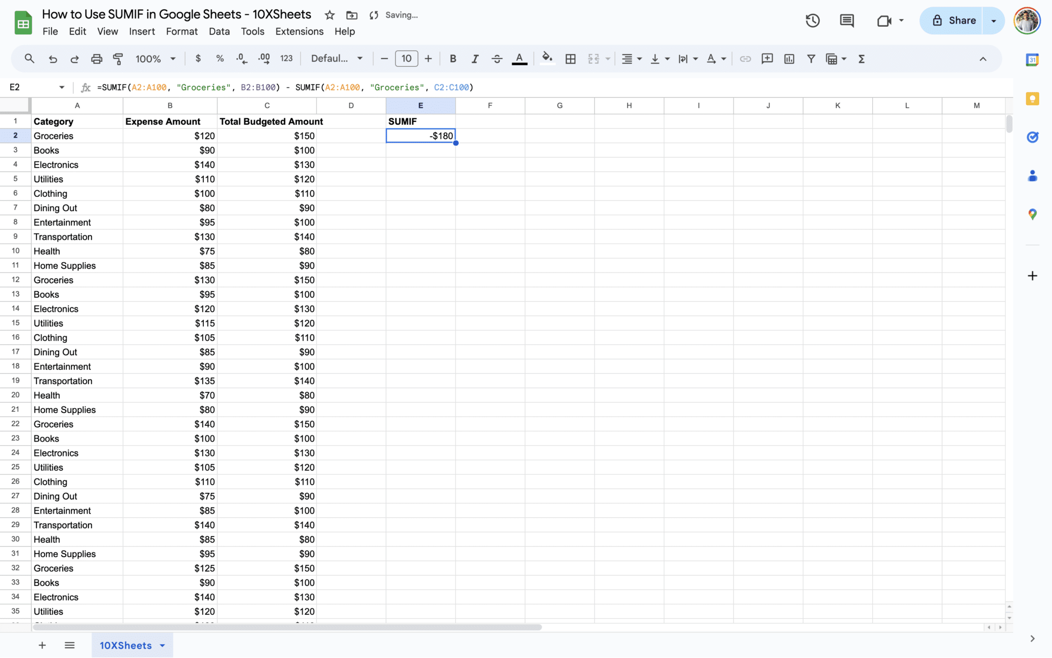
By comparing actual expenses with budgeted amounts using SUMIF, you can identify areas where you may be overspending and adjust your budget accordingly to achieve your financial goals.
Google Sheets SUMIF Tips and Best Practices
Let's explore some tips and best practices to enhance your usage of the SUMIF function in Google Sheets. These practices will help you keep your formulas concise, organize your data efficiently, and troubleshoot common issues effectively.
Keeping SUMIF Formulas Concise and Readable
When working with SUMIF formulas, it's essential to keep them concise and easy to understand. This not only improves readability but also makes it easier to troubleshoot and maintain your spreadsheets in the long run.
Here are some tips for keeping your SUMIF formulas concise and readable:
-
Use Descriptive Cell References: Instead of referencing individual cells directly in your formula, use descriptive cell references or named ranges. This makes it easier to understand the purpose of each part of the formula.
-
Break Down Complex Formulas: If your SUMIF formula becomes too complex, consider breaking it down into smaller, more manageable parts. You can use helper columns or intermediate calculations to simplify complex logic.
-
Use Comments: Add comments to your formulas to provide context and explanation for future reference. This can be especially helpful when sharing spreadsheets with others or revisiting them later.
By following these practices, you can create SUMIF formulas that are easy to understand and maintain, even as your spreadsheet grows in complexity.
Organizing Data for Efficient SUMIF Usage
To make the most of the SUMIF function, it's crucial to organize your data efficiently within your spreadsheet. Proper data organization simplifies the process of applying SUMIF formulas and ensures accurate results.
Here are some tips for organizing your data for efficient SUMIF usage:
-
Consistent Data Formatting: Ensure that data within your ranges is formatted consistently. This includes using the same units, date formats, and text conventions throughout your dataset.
-
Group Related Data Together: Group related data together within your spreadsheet to make it easier to reference in your SUMIF formulas. For example, keep all sales data in one section and expense data in another.
-
Sort Data Appropriately: Sort your data in a logical order based on the criteria you plan to use with SUMIF. This can help improve the performance of your formulas and make it easier to locate specific data points.
By organizing your data thoughtfully, you can streamline the process of applying SUMIF formulas and ensure accurate results in your analysis.
Debugging Common Issues in SUMIF Formulas
Despite your best efforts, you may encounter errors or unexpected results when using SUMIF formulas. Knowing how to debug common issues can help you identify and resolve problems quickly.
Here are some common issues you may encounter with SUMIF formulas and how to debug them:
-
Incorrect Criteria: Double-check the criteria you're using in your SUMIF formula. Ensure that it matches the data format and is spelled correctly. Use the "Evaluate Formula" tool in Google Sheets to see how the formula is being evaluated step by step.
-
Mismatched Ranges: Verify that the ranges you're using in your SUMIF formula are aligned correctly. Ensure that the range containing the criteria matches the range containing the values to be summed.
-
Data Type Mismatch: Check for data type mismatches between the criteria and the values in your SUMIF formula. For example, if you're comparing text criteria with numeric values, ensure they're compatible.
By diligently debugging common issues in your SUMIF formulas, you can maintain the accuracy and reliability of your spreadsheet calculations.
Conclusion
Mastering the SUMIF function in Google Sheets opens up a world of possibilities for data analysis and manipulation. By understanding its syntax, parameters, and various applications, you can streamline your workflow and extract valuable insights from your datasets with ease. Whether you're a business professional analyzing sales data, a student tracking expenses, or a budget-conscious individual managing personal finances, SUMIF is a versatile tool that empowers you to make informed decisions based on accurate data.
Furthermore, by incorporating advanced techniques such as nesting SUMIF with other functions, using logical operators, and employing wildcards, you can take your spreadsheet skills to the next level. These techniques allow for more complex calculations and provide greater flexibility in handling diverse datasets. With practice and experimentation, you'll become proficient in harnessing the full potential of SUMIF, enhancing your productivity and effectiveness in Google Sheets.
Frequently asked questions
What is the SUMIF Function in Google Sheets?
The SUMIF function in Google Sheets is a powerful tool that allows you to perform conditional summations based on specific criteria. It simplifies the process of summarizing data by summing only the values that meet certain conditions, thereby providing valuable insights into your dataset. Understanding how to use SUMIF effectively can significantly enhance your ability to analyze and manipulate data within Google Sheets.
How to Use SUMIF in Google Sheets?
Let's explore some fundamental ways to apply the SUMIF function for simple calculations and how you can utilize cell references to enhance the flexibility of your formulas.