How to Freeze a Row in Google Sheets? (A 2024 Guide)

Ever found yourself scrolling endlessly through a massive Google Sheets spreadsheet, losing track of those crucial headers or vital data points? You’re not alone. The question is, how can you make your Google Sheets experience smoother and more efficient? The answer lies in mastering the art of freezing rows and columns. In this guide, we’ll unravel the secrets of freezing rows and columns in Google Sheets, empowering you to effortlessly keep your essential data within reach, no matter how vast your spreadsheet may be.

What is Freezing a Row in Google Sheets?

Freezing a row in Google Sheets refers to the practice of pinning a specific row at the top of your spreadsheet, ensuring that it remains visible as you scroll down through your data. Essentially, frozen rows stay fixed in place, creating a helpful reference point that keeps important information readily accessible, even when dealing with extensive spreadsheets.

Key Points about Freezing Rows:

1. Row Position: When you freeze a row, it remains at the top of your spreadsheet, regardless of how far down you scroll. This is especially valuable when your spreadsheet contains headers, titles, or any critical data you need to see continuously.
2. Scrolling Efficiency: Freezing rows enhances your scrolling efficiency, as you can quickly refer back to the frozen row for context or comparison while examining data further down the sheet.
3. Header Visibility: For tables with column headers, freezing the top row ensures that column titles remain visible, making it easy to understand the content of each column.
4. Easy Navigation: It simplifies navigation within large datasets, eliminating the need to constantly scroll up to review essential details.
5. Customizable: Google Sheets allows you to freeze not just one row but multiple rows at the top of your sheet, catering to your specific needs.

Importance of Freezing Rows in Google Sheets

Freezing rows in Google Sheets is essential for several reasons, especially when working with complex or extensive datasets:

1. Maintaining Context: When dealing with large spreadsheets, it’s easy to lose context as you scroll. Freezing rows ensures that crucial context, such as headers or labels, remains in view, preventing data misinterpretation.
2. Data Comparison: Freezing rows enables easy comparison of data in different parts of the sheet. You can effortlessly cross-reference information in the frozen row with data further down in the spreadsheet.
3. Efficient Data Entry: If you’re inputting data into a lengthy spreadsheet, freezing rows with input fields or dropdown menus can streamline the data entry process. You can always see the input fields as you move through the sheet.
4. Data Analysis: When performing data analysis, it’s vital to have quick access to data headers and relevant information. Freezing rows facilitates data analysis by providing instant access to critical data points.
5. User-Friendly Viewing: Freezing rows improves the user experience for anyone accessing your spreadsheet. It reduces the need for constant scrolling, making it easier for collaborators or stakeholders to navigate and understand the data.
6. Better Presentation: If you plan to share your spreadsheet with others or use it for presentations, frozen rows ensure that essential information is consistently visible, enhancing the overall presentation quality.

In summary, freezing rows in Google Sheets is a valuable feature that enhances usability, efficiency, and comprehension when working with large or complex datasets. It ensures that critical information remains within your field of view, making your spreadsheet more user-friendly and productive.

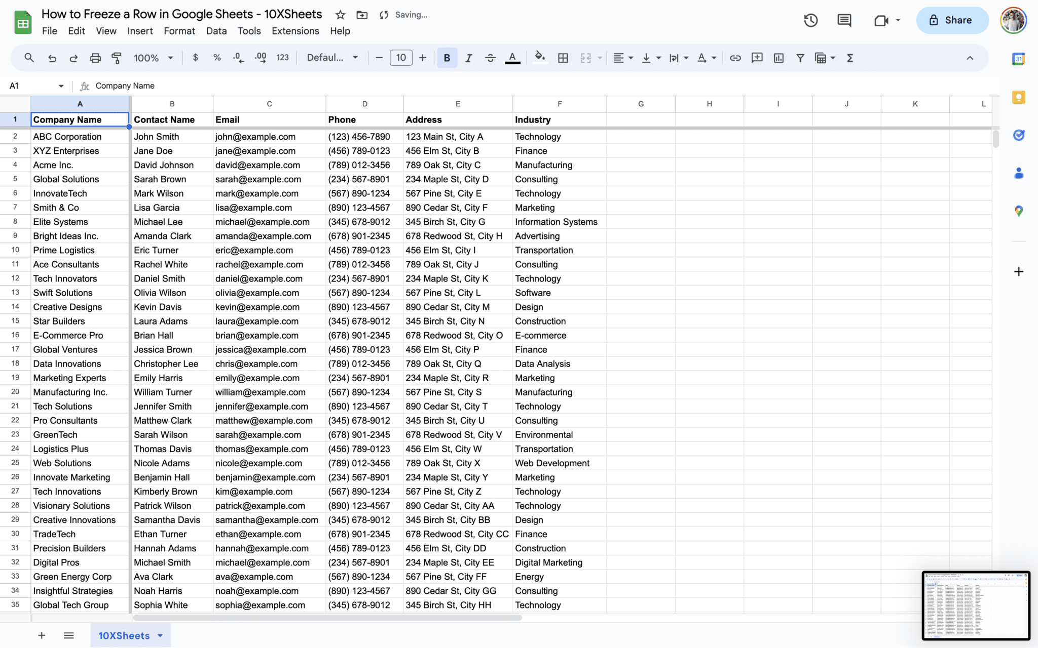
Understanding Google Sheets Rows and Columns

When working with Google Sheets, it’s crucial to understand the fundamental building blocks of your spreadsheet: rows, columns, and cell references. In this section, we’ll delve deeper into each of these elements to provide you with a solid foundation for freezing rows and columns effectively.

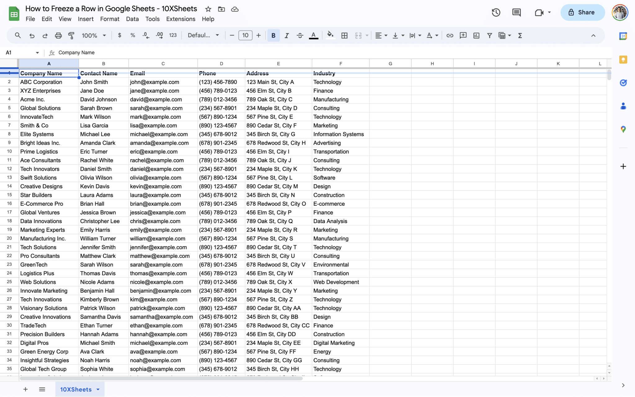
1. Rows in Google Sheets

Rows in Google Sheets are the horizontal sections that run from left to right across your spreadsheet. Each row is identified by a unique number, starting with 1 for the topmost row, 2 for the next, and so on. Rows are used to organize and group data horizontally.

Key Points about Rows:

• Rows are numbered sequentially, making it easy to reference specific rows within your spreadsheet.
• Each row contains cells, which are the individual boxes where you enter and display data.
• Rows are essential for organizing data in a structured manner, especially when dealing with large datasets.

2. Columns in Google Sheets

Columns in Google Sheets are the vertical sections that run from top to bottom. Unlike rows, columns are labeled with letters, starting with ‘A’ for the first column, ‘B’ for the second, and continuing through the alphabet. Columns are used to organize and categorize data vertically.

Key Points about Columns:

• Columns are labeled alphabetically, making it easy to reference specific columns within your spreadsheet.
• Each column contains cells that hold data, text, numbers, or formulas.
• Columns are instrumental in structuring your data and facilitating calculations, as they allow you to work with data in a vertical format.

3. Cell References

In Google Sheets, cell references are the addresses used to identify and locate a specific cell within a spreadsheet. A cell reference consists of a combination of a column letter and a row number, such as ‘A1,’ ‘B5,’ or ‘C12.’ Understanding cell references is essential when you need to work with data across different cells or perform calculations.

Key Points about Cell References:

• Cell references are used in formulas and functions to perform calculations and manipulate data.
• They are written in a format that combines a column letter and a row number, allowing you to pinpoint a particular cell.
• Absolute and relative cell references provide flexibility in how you reference cells within your formulas.

In summary, a solid grasp of rows, columns, and cell references is fundamental to effectively navigating and working with data in Google Sheets. As you proceed with freezing rows and columns, keep in mind how these foundational elements interact and play a crucial role in structuring your spreadsheets.

How to Freeze Rows and Columns in Google Sheets?

Now, let’s explore the various methods for freezing rows and columns in Google Sheets. Freezing specific rows or columns is incredibly useful when dealing with extensive spreadsheets, as it keeps important data visible as you scroll. We’ll cover three different methods for achieving this: the Drag & Drop Shortcut, using the View Menu, and the Right-Click Menu.

1. How to Freeze a Row or Column in Google Sheets Using the Drag & Drop Shortcut?

The Drag & Drop Shortcut is one of the quickest ways to freeze rows and columns in Google Sheets. It provides a visual and intuitive way to keep your desired rows or columns in view.

Using the Drag & Drop Method

To freeze rows or columns using the Drag & Drop Method:

1. Hover your cursor over the empty square where the row headers and column headers intersect.
2. To freeze a row, hover over the bottom line of the square until it’s highlighted.
3. Click and drag the outline downward to go beyond the row you want to freeze.
4. No matter how far down you scroll, the first rows will stay visible.

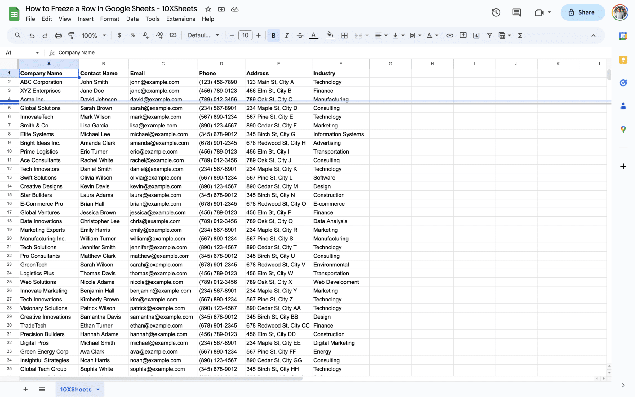
Freezing the Top Row

To freeze the top row using the Drag & Drop Shortcut:

1. Hover your cursor over the empty square where the row headers and column headers intersect.
2. To freeze the top row, hover over the bottom line of the square until it’s highlighted.
   
3. Click and drag the outline downward just beyond the top row.
   

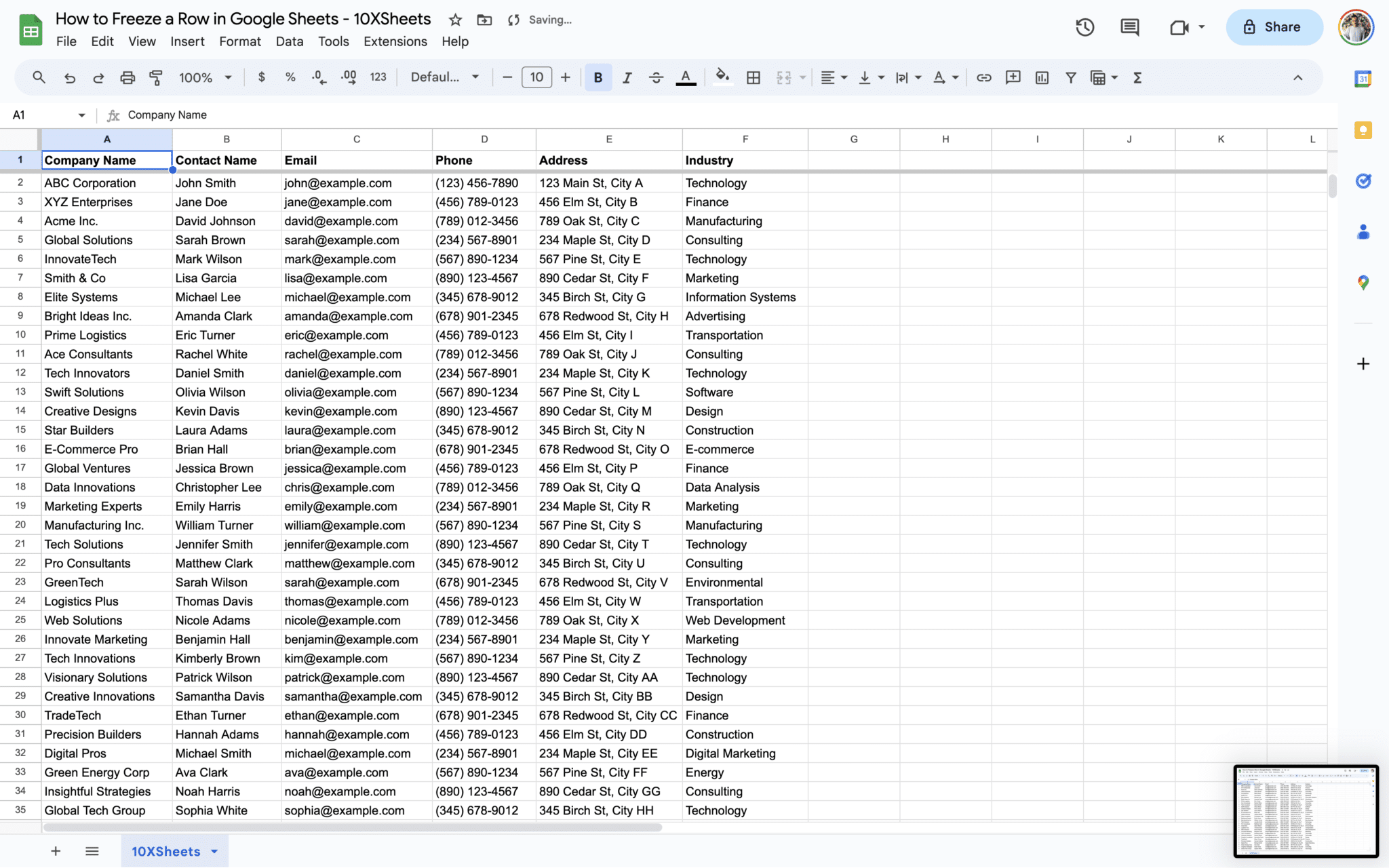
Now, as you scroll down, the top row will remain in view, providing constant access to your column headers.

Freezing the First Column

To freeze the first column using the Drag & Drop Shortcut:

1. Hover your cursor over the empty square where the row headers and column headers intersect.
2. To freeze the first column, hover over the left-hand line of the square until it’s highlighted.
   
3. Click and drag the outline to the right just beyond the first column.
   

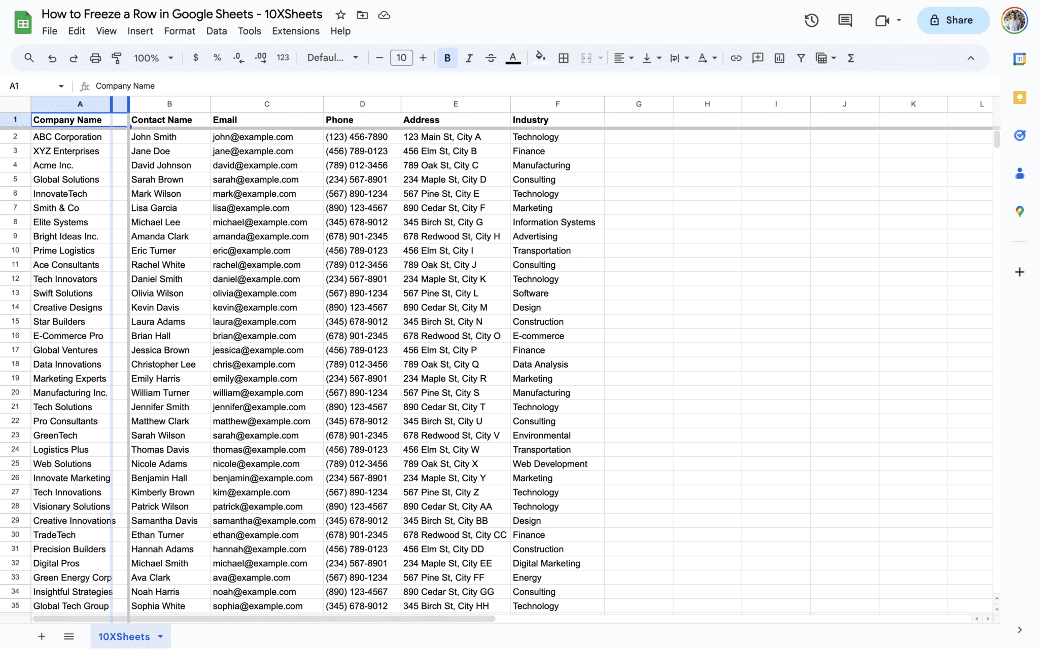
Now, no matter how far to the right you scroll, the first column will always be visible, ensuring easy reference to your row headers.

2. How to Freeze a Row or Column in Google Sheets using the View Menu?

Using the View Menu offers precise control over which rows or columns to freeze in Google Sheets.

Freezing Rows via View Menu

To freeze rows via the View Menu:

1. Click on the View menu located at the top of the Google Sheets interface.
2. Choose Freeze from the dropdown menu.
3. Select ‘1 row’ to freeze the top row or ‘2 rows’ to freeze the top two rows.
   

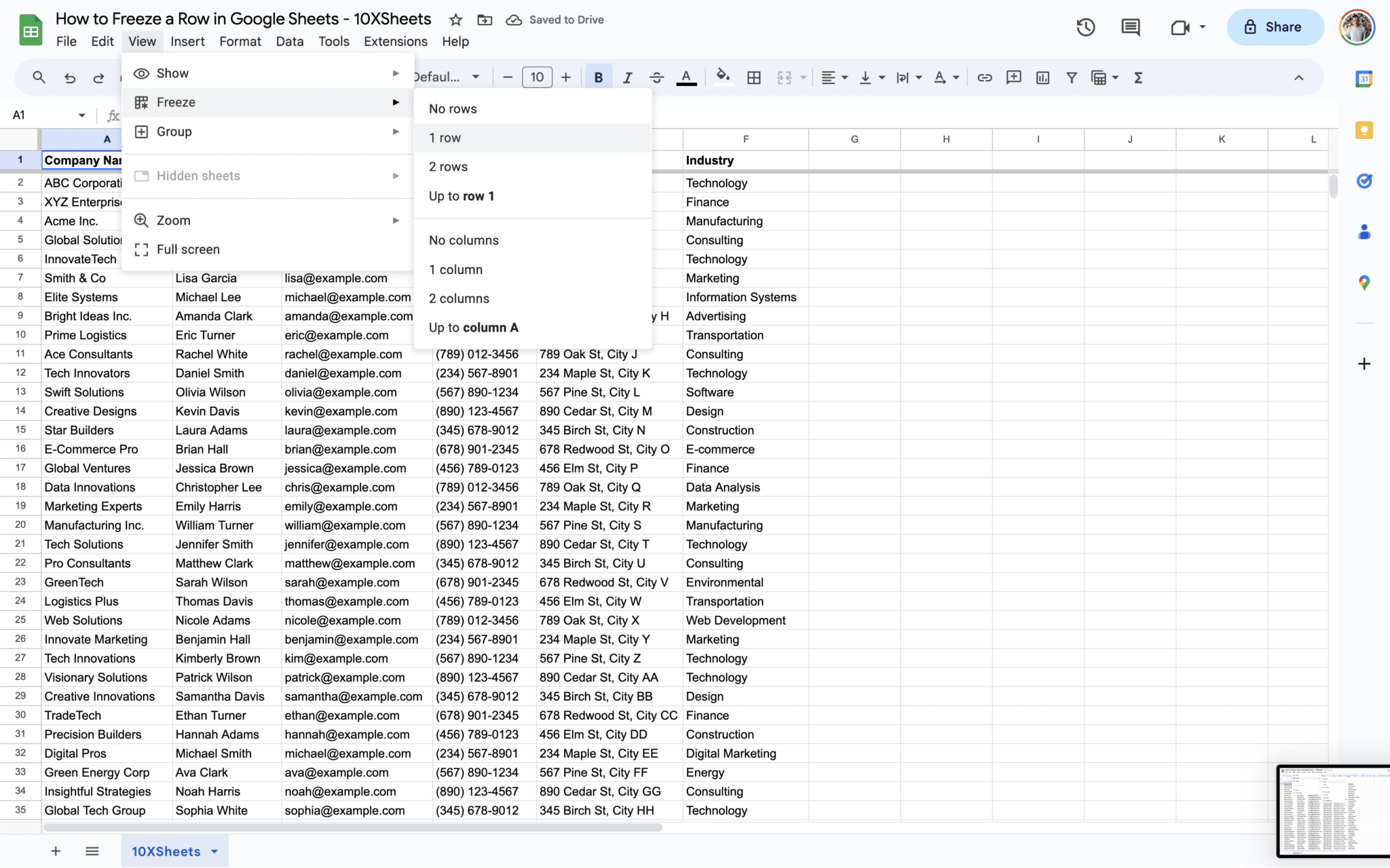
Now, the selected rows will remain visible as you scroll through your spreadsheet.

Freezing Columns via View Menu

To freeze columns via the View Menu:

1. Click on the View menu.
2. Choose Freeze from the dropdown menu.
3. Select ‘1 column’ to freeze the first column or ‘2 columns’ to freeze the first two columns.
   

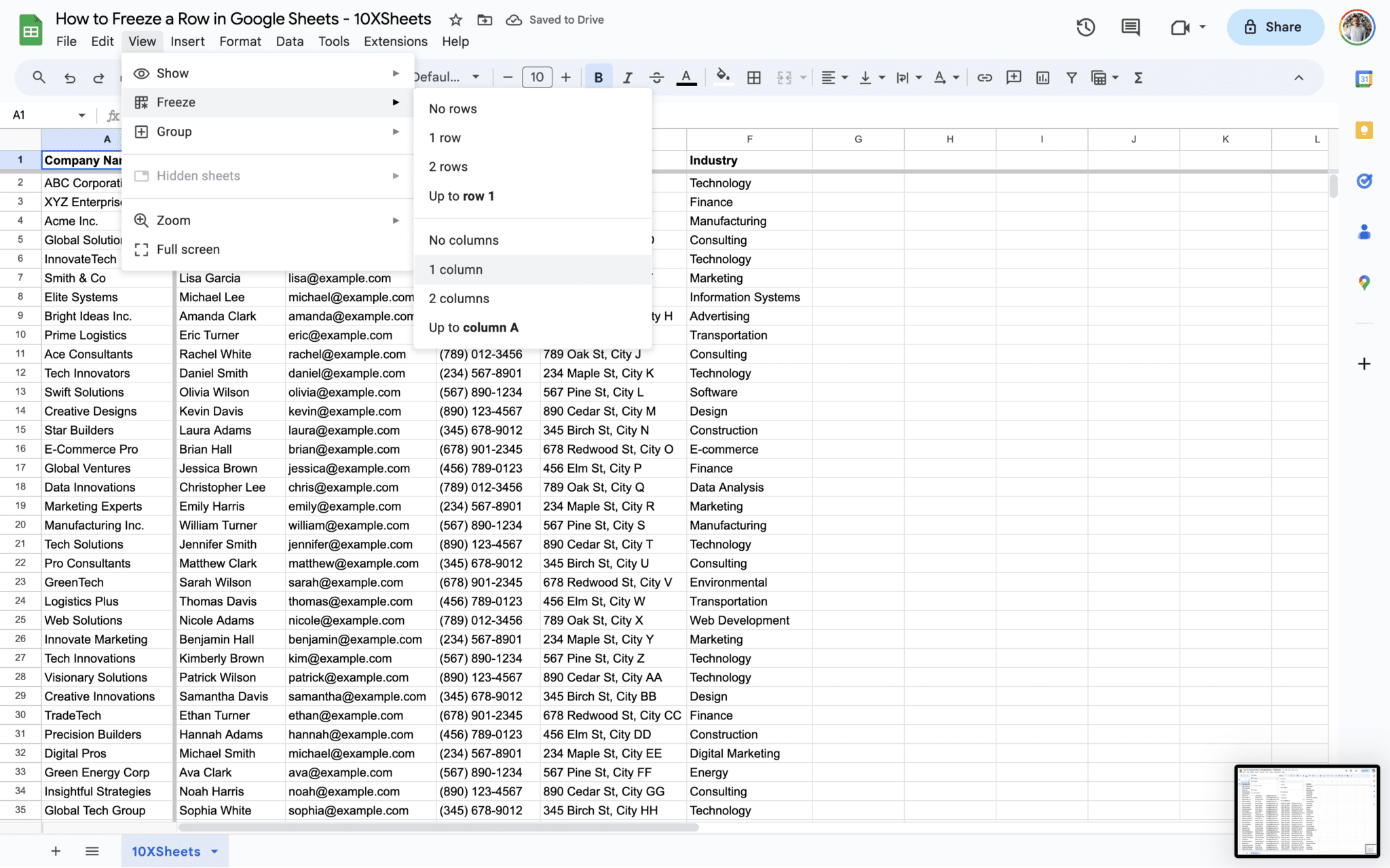
This will ensure that the chosen columns remain in view as you navigate horizontally through your spreadsheet.

3. How to Freeze a Row or Column in Google Sheets using the Right-Click Menu?

The Right-Click Menu provides a convenient way to freeze rows and columns by simply right-clicking on your desired row or column.

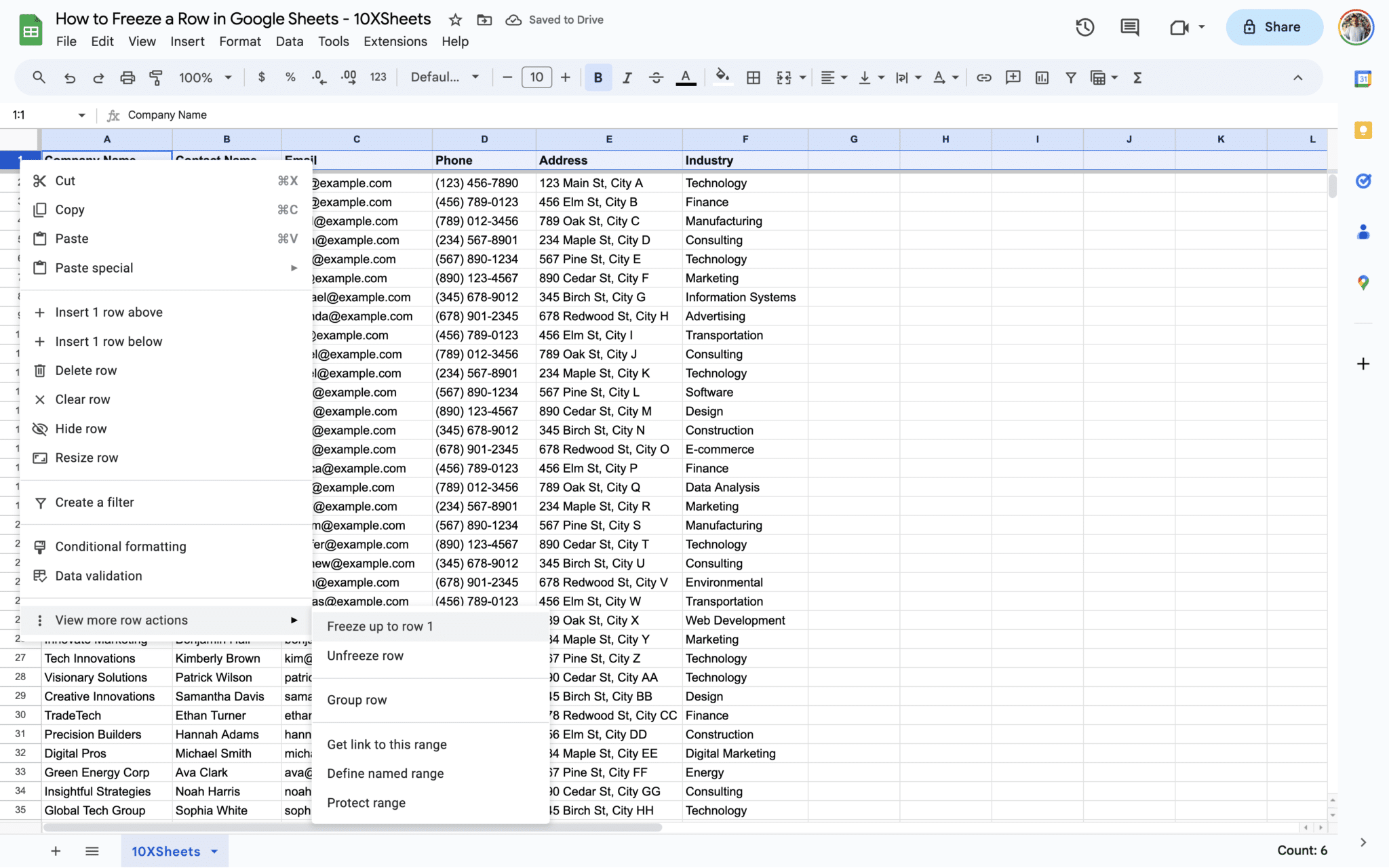
Freezing Rows via Right-Click Menu

To freeze rows via the Right-Click Menu:

1. Select the row you want to freeze by clicking on the row number.
2. Right-click on the selected row number to open the context menu.
3. From the menu, navigate to View more row actions and select Freeze up to row 1 to freeze the chosen row.
   

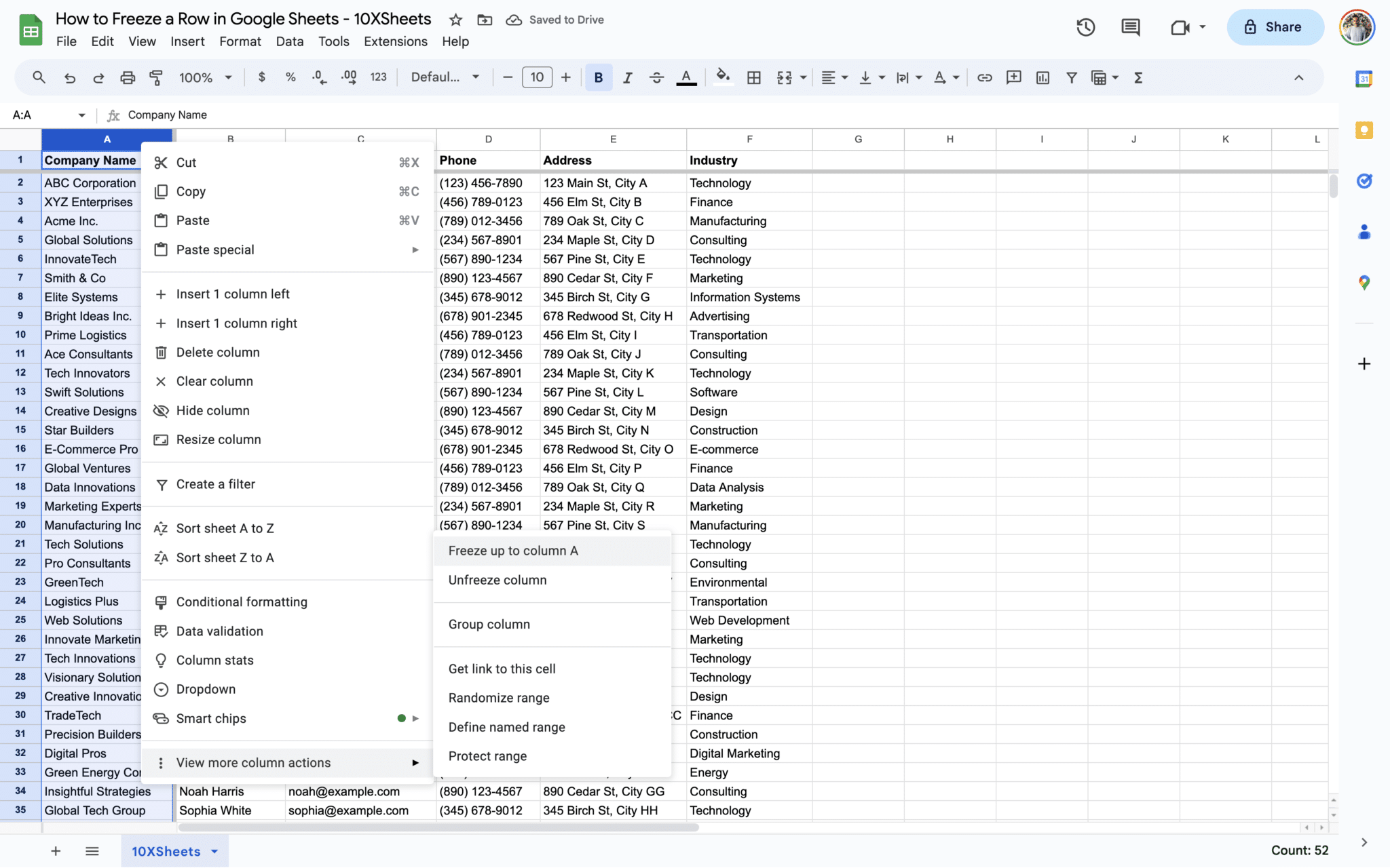
Freezing Columns via Right-Click Menu

To freeze columns via the Right-Click Menu:

1. Select the column you want to freeze by clicking on the column letter.
2. Right-click on the selected column letter to open the context menu.
3. From the menu, go to View more column actions and choose Freeze up to column A to freeze the selected column.
   

These simple right-click actions give you the flexibility to freeze rows and columns with ease.

With these three methods at your disposal, you can choose the one that best suits your workflow and spreadsheet structure. Whether you prefer a visual approach, precise menu selections, or right-click convenience, Google Sheets offers versatile options for keeping your important data in view while working with large datasets.

How to Freeze Multiple Rows and Columns in Google Sheets?

In Google Sheets, you often need to freeze not just a single row or column but multiple rows and columns to keep your spreadsheet organized and easy to navigate. This section will guide you through the process of freezing multiple rows and columns using various methods.

1. How to Freeze Multiple Rows and Columns Using Drag & Drop?

To freeze multiple rows and columns using the Drag & Drop method:

1. Hover your cursor over the empty square where the row headers and column headers intersect.
2. To freeze multiple rows, hover over the bottom line of the square until it’s highlighted.
3. Click and drag the outline downward to encompass the rows you want to freeze.
   

Example: If you want to freeze the first four rows, drag the outline beyond the fourth row.

4. To freeze multiple columns, repeat the same process, but this time, hover over the left-hand line of the square and drag it to include the columns you want to freeze.
   

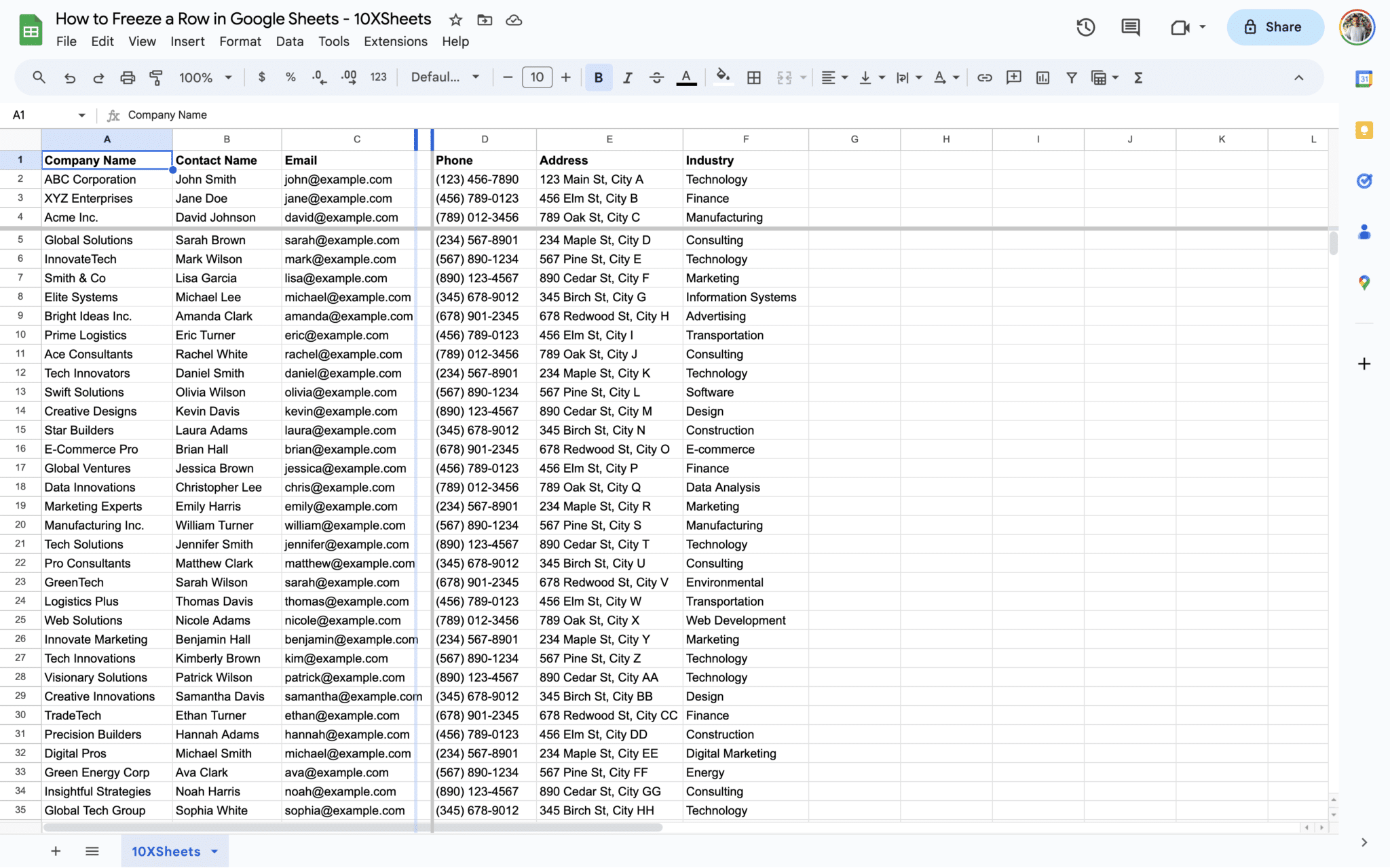
By using this method, you can easily freeze both rows and columns simultaneously, providing you with a customized view of your data.

2. How to Freeze Multiple Rows and Columns via View Menu?

Freezing multiple rows and columns via the View Menu provides a precise and straightforward way to control which parts of your spreadsheet remain visible as you scroll.

1. Click on the View menu located at the top of the Google Sheets interface.
2. Choose Freeze from the dropdown menu.
3. Select ‘1 row’ to freeze the top row or ‘2 rows’ to freeze the top two rows. Likewise, you can choose ‘1 column’ or ‘2 columns’ to freeze the first one or two columns.
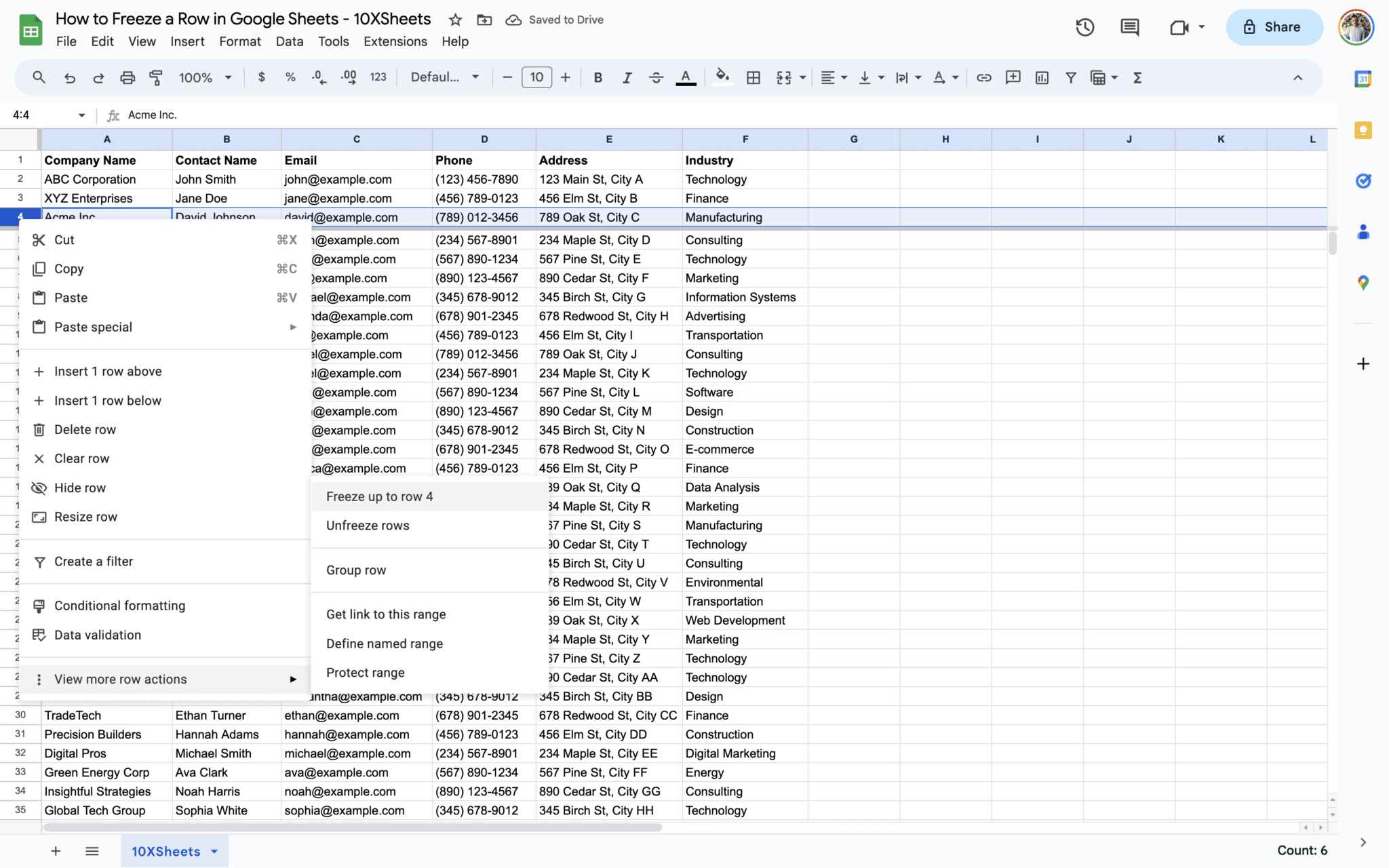
4. To freeze multiple rows, select a cell from the row or column you want to freeze and go back to View > Freeze > up to row/column X. For example, select cell D4 and head to View > Freeze. Then, select up to row 4 to freeze the first 4 rows.
   
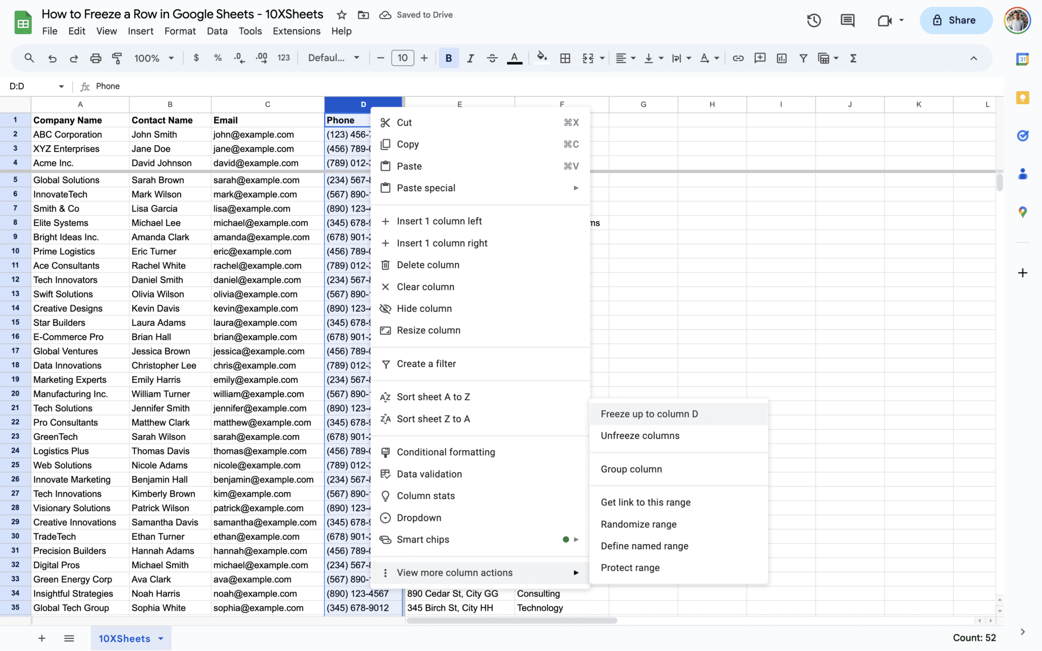
5. Similarly, you can select up to column D to freeze the first 4 columns.

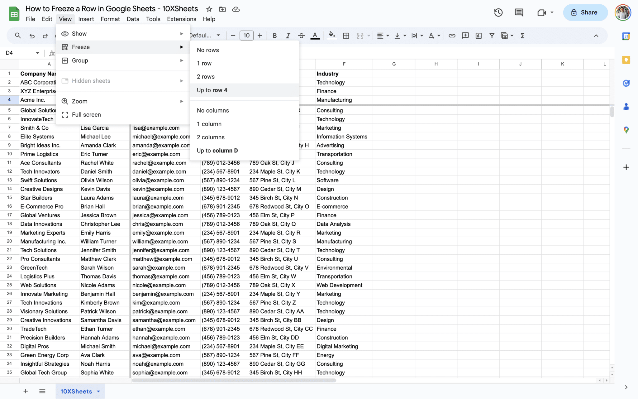
Using this method, you can precisely specify the number of rows and columns to freeze, allowing you to maintain visibility over more extensive portions of your spreadsheet.

3. How to Freeze Multiple Rows and Columns via Right-Click Menu?

The Right-Click Menu offers an efficient way to freeze multiple rows and columns with just a few clicks.

To freeze multiple rows via Right-Click Menu:

1. Select the first row you want to freeze by clicking on its row number.
2. Right-click on the selected row number to open the context menu.
3. From the menu, navigate to View more row actions and select Freeze up to row X, where X is the last row you want to freeze.
   
4. Repeat these steps if you wish to freeze additional rows.

To freeze multiple columns via Right-Click Menu:

1. Select the first column you want to freeze by clicking on its column letter.
2. Right-click on the selected column letter to open the context menu.
3. From the menu, go to View more column actions and choose Freeze up to column Y, where Y is the last column you want to freeze.
   
4. Repeat these steps if you wish to freeze additional columns.

This method allows you to efficiently freeze multiple rows and columns, giving you greater control over your spreadsheet’s structure.

How to Freeze Rows and Columns in the Google Sheets Mobile App?

If you’re using the Google Sheets mobile app, you can still freeze rows and columns to make working with your spreadsheets more manageable. Here, we’ll explore two methods for freezing rows and columns directly from your mobile device.

1. Freezing Rows or Columns from Row or Column Header

1. In the Google Sheets mobile app, open the spreadsheet you want to work on.
2. To freeze a row, tap on the row number that you want to freeze. Similarly, to freeze a column, tap on the column letter you wish to freeze.
3. After tapping the row or column header, a menu will appear.
4. From the menu, select ‘Freeze row’ to freeze the row or ‘Freeze column’ to freeze the column.

Now, the chosen row or column will stay in view, making it easier for you to reference important data as you scroll through your spreadsheet on your mobile device.

2. Freezing Rows or Columns from Tab or Sheet Name

1. Open the Google Sheets mobile app and access your spreadsheet.
2. Tap on the tab or sheet name at the bottom of the screen to open the menu.
3. In the menu, use the arrows or options provided to specify the number of rows and columns you want to freeze.
4. Adjust the settings according to your preferences and confirm your selection.

By using this method, you can easily freeze rows and columns in the Google Sheets mobile app, ensuring that your crucial data remains accessible and visible, even when working on a smaller screen.

Tips and Tricks for Freezing Rows and Columns in Google Sheets

Now that you’ve learned how to freeze rows and columns effectively in Google Sheets, let’s explore some valuable tips and tricks to make the most of this feature.

Making the Most of Frozen Rows and Columns

Freezing rows and columns is a powerful tool, but maximizing its utility requires a few additional strategies:

1. Use Freeze Panes for Header Rows: When dealing with large datasets, it’s common to have multiple header rows. To keep all important headers visible, consider freezing multiple rows at the top of your sheet. This ensures that as you scroll down, all relevant header information remains in view.
2. Freeze Key Data Columns: In addition to freezing the top row, you can freeze one or more key data columns. This is especially useful when working with complex data sets, as it allows you to compare data in different columns without losing context.
3. Combine Freezing with Filters: You can enhance your data analysis by using filters in Google Sheets. When you freeze rows and columns along with filters, you can easily sort and filter data without losing sight of your headers or crucial reference points.
4. Utilize Split and Freeze: Google Sheets offers a split and freeze feature that allows you to freeze both rows and columns simultaneously. This feature is handy when you want to keep a specific section of your spreadsheet constantly in view while navigating through your data.
5. Consider Mobile Usability: If you anticipate accessing your Google Sheets on mobile devices, keep in mind that freezing rows and columns is equally effective on mobile apps. Adjust your freezing settings to optimize the mobile viewing experience.

Troubleshooting Common Issues

While freezing rows and columns is relatively straightforward, you may encounter some common issues. Here are solutions to address these problems:

1. Overlapping Freeze Panes: If you freeze both rows and columns and they overlap, it can create confusion. To resolve this, unfreeze the conflicting rows or columns and reapply the freezing according to your requirements.
2. Hidden Rows or Columns: When you freeze rows or columns, any hidden rows or columns within the frozen area may cause unexpected results. Ensure that you unhide any rows or columns you need before applying freezing.
3. Freeze Not Working on Mobile App: If you’re having trouble freezing rows or columns in the mobile app, ensure that you are tapping the correct row or column headers to access the freezing options. Double-check your selections and try again.
4. Frozen Area Limits: Google Sheets has limitations on the number of rows and columns you can freeze. If you’re unable to freeze as much as you need, consider other ways to organize your spreadsheet, such as grouping rows or columns.

Best Practices for Using Frozen Rows and Columns

To make the most of frozen rows and columns, follow these best practices:

1. Plan Your Spreadsheet Structure: Before applying freezing, think about your data and how it should be organized. Careful planning ensures that you freeze the right rows and columns for your specific needs.
2. Keep It Simple: Avoid freezing too many rows or columns, as it can clutter your view. Freeze only what is necessary to maintain clarity and visibility.
3. Regularly Review and Adjust: As your spreadsheet evolves, periodically review your freezing settings. You may need to adjust them to accommodate changes in your data or analysis requirements.
4. Document Your Freezing Choices: If you’re working with others on the same spreadsheet, document the rows and columns you’ve frozen to ensure everyone understands the structure.

By implementing these tips, troubleshooting issues, and following best practices, you’ll be able to harness the full potential of frozen rows and columns in Google Sheets to streamline your data management and analysis tasks.