Get Started With a Prebuilt Model

Start with a free template and upgrade when needed.

Are you ready to master the art of data manipulation and calculation in Google Sheets? Dive into the world of spreadsheet sorcery as we unveil the secrets behind the top Google Sheets formulas.

In this guide, you’ll learn how to harness the power of these formulas to streamline your data-driven tasks, analyze information with precision, and unleash the full potential of Google Sheets. Whether you’re a beginner seeking to build a strong foundation or an experienced user looking to level up your skills, our guide will equip you with the knowledge and tools you need to excel in the realm of spreadsheets.

What are Google Sheets Formulas?

Google Sheets formulas are mathematical or logical expressions used within Google Sheets, a cloud-based spreadsheet application, to perform calculations, manipulate data, and automate tasks. These formulas enable users to perform a wide range of operations, from basic arithmetic calculations to complex data analysis and manipulation. They typically consist of predefined functions, operators, and cell references, allowing users to process and interpret data, make informed decisions, and create dynamic reports within their spreadsheets.

Google Sheets formulas are essential tools for efficiently managing, analyzing, and deriving insights from data in various personal, educational, and professional settings.

Components of a Google Sheets Formula

A typical Google Sheets formula consists of three main components:

  1. Function: The function is the core of the formula and determines the type of calculation or operation to be performed. Functions are predefined by Google Sheets and cover a wide range of tasks, from basic arithmetic to complex data analysis.
  2. Arguments: Arguments are the inputs provided to the function. These can be numbers, cell references, text, or other values that the function operates on. Functions may require one or more arguments, depending on their purpose.
  3. Operators: Operators are symbols that dictate how the formula’s elements should interact. Common operators include addition (+), subtraction (-), multiplication (*), and division (/).

For example, the formula =SUM(A1:A5) uses the SUM function to add the values in cells A1 through A5. In this case, A1:A5 is the argument, and the SUM function performs the addition operation.

Importance of Formulas in Google Sheets

Formulas are the driving force behind the functionality and versatility of Google Sheets. Here’s why they are crucial:

  1. Automation: Formulas automate repetitive tasks, eliminating the need for manual calculations and data entry. This saves time and reduces the risk of errors.
  2. Data Analysis: Formulas enable you to analyze and interpret data in various ways, from simple calculations to complex statistical analysis. You can generate insights and make informed decisions based on your data.
  3. Dynamic Updates: Formulas ensure that your spreadsheet remains up-to-date. When you change the input data, formulas recalculate automatically, providing real-time results.
  4. Consistency: Formulas enforce consistency by applying the same calculations or rules to multiple data points. This reduces inconsistencies and maintains data integrity.
  5. Customization: You can create custom formulas to meet specific requirements. Google Sheets offers a variety of built-in functions, and you can even develop your own custom functions using JavaScript.

How to Get Started with Google Sheets Formulas?

Before diving into the world of Google Sheets formulas, it’s essential to have a basic understanding of the application itself. Here are some fundamental steps to get you started:

  1. Access Google Sheets: Open your web browser and navigate to Google Sheets by visiting sheets.google.com.
  2. Sign In or Create an Account: Sign in with your Google account or create one if you don’t have it.
  3. Create a New Spreadsheet: Click on the “Blank” option to start a new spreadsheet. You’ll be presented with a blank grid where you can enter your data and formulas.
  4. Entering Data: Begin by entering your data into the cells. Each cell can contain text, numbers, dates, or formulas.
  5. Creating Formulas: To create a formula, select the cell where you want the result to appear and start typing your formula using the equal sign (=) followed by the function name and arguments. You can also click on functions from the “Functions” menu to insert them into the formula bar.
  6. Cell References: Make use of cell references in your formulas. Instead of hardcoding values, refer to cell addresses for dynamic calculations.
  7. Testing and Debugging: Test your formulas to ensure they produce the desired results. If you encounter errors, use Google Sheets’ error-checking tools and the formula auditing feature to identify and resolve issues.

Understanding the basics of Google Sheets and the significance of formulas is the first step towards becoming proficient in spreadsheet management and data analysis. As you become more familiar with these concepts, you can explore more advanced formula techniques and functions to unlock the full potential of Google Sheets.

Basic Google Sheets Functions

Now, let’s delve deeper into the fundamental building blocks of Google Sheets—basic functions. These functions are the backbone of any spreadsheet, empowering you to perform essential calculations, summarize data, and gain meaningful insights. We will explore four crucial basic functions: SUM, AVERAGE, MAX, and MIN, along with COUNT and COUNTA for effective data counting.

SUM Function

The SUM function is your trusty companion for adding up numbers within a given range. Its versatility extends to a wide array of applications, from totaling expenses in a monthly budget to calculating the sales revenue for a specific period.

Here’s how to use the SUM function in Google Sheets:

=SUM(range)

Where ‘range’ represents the cells you want to sum up. For example, imagine you have a sales dataset in cells A1 to A10. To calculate the total sales for this period, simply enter:

=SUM(A1:A10)

The SUM function instantly computes the sum, saving you valuable time and minimizing the chances of manual errors in your calculations.

AVERAGE Function

The AVERAGE function steps in when you need to find the mean or average value of a set of numbers. Whether you’re analyzing test scores, product ratings, or employee performance, AVERAGE simplifies the process.

Here’s the AVERAGE function in action:

=AVERAGE(range)

For example, suppose you want to determine the average score of students in cells B1 to B20. You’d use:

=AVERAGE(B1:B20)

AVERAGE computes the mean, allowing you to gauge the central tendency of your data. This is particularly useful for identifying trends and making data-driven decisions.

MAX and MIN Functions

The MAX and MIN functions are indispensable when you need to identify the highest and lowest values within a dataset. Whether you’re tracking stock prices, monitoring temperature fluctuations, or evaluating performance metrics, these functions help you pinpoint peaks and valleys.

  • MAX Function: This function returns the largest value in a given range. Here’s how to apply it:
    =MAX(range)

    Let’s say you have a list of daily temperatures in cells C1 to C30. To find the highest temperature recorded during the month, use:

    =MAX(C1:C30)
  • MIN Function: Conversely, the MIN function locates the smallest value within a range. It’s structured as follows:
    =MIN(range)

    To discover the lowest temperature from the same dataset, you’d utilize:

    =MIN(C1:C30)

The MAX and MIN functions are invaluable for quick data analysis and help you recognize extremes within your dataset. Whether you’re identifying the hottest day of the year or the lowest stock price in a given period, these functions provide instant answers.

COUNT and COUNTA Functions

Counting data is a fundamental operation in spreadsheet work. The COUNT and COUNTA functions come to your aid when you need to tally the number of items in a list or count non-empty cells.

  • COUNT Function: It counts the number of cells containing numerical values within a specified range. The formula structure is straightforward:
    =COUNT(range)

    For instance, suppose you want to count the number of products sold in cells D1 to D50. Simply employ:

    =COUNT(D1:D50)
  • COUNTA Function: COUNTA takes a broader approach by counting all non-empty cells within a range, regardless of their content. It’s used like this:
    =COUNTA(range)

    To determine the number of filled cells in a list of customer names in cells E1 to E100, you’d utilize:

    =COUNTA(E1:E100)

These functions play a pivotal role in data validation and cleanliness. Whether you’re checking for missing data points, assessing the completeness of a survey, or tracking inventory levels, COUNT and COUNTA are indispensable tools for maintaining data integrity

Google Sheets Mathematical Functions

Now, let’s embark on a journey through the realm of mathematical functions in Google Sheets. These functions empower you to perform a wide range of arithmetic operations and manipulate numeric data with precision. We’ll explore three key areas of mathematical functions: Addition and Subtraction, Multiplication and Division, and Exponents and Square Roots.

Addition and Subtraction

Addition and Subtraction are the fundamental building blocks of mathematics, and they’re just as vital in Google Sheets. These operations allow you to combine and subtract values, making them invaluable for various spreadsheet tasks.

Addition

Adding numbers in Google Sheets is as simple as using the + operator. For example:

=A1 + B1

This formula adds the values in cells A1 and B1. You can also add multiple cells or constant values together in a similar fashion.

Subtraction

Subtraction follows a similar pattern. Use the - operator to subtract one value from another:

=C1 - D1

This formula subtracts the value in cell D1 from the value in cell C1. As with addition, you can perform subtraction with multiple cells or constants.

Multiplication and Division

Multiplication and Division are essential for various tasks, such as calculating total costs, determining average prices, or forecasting growth.

Multiplication

To multiply values in Google Sheets, use the * operator:

=E1 * F1

This formula multiplies the values in cells E1 and F1 together. You can multiply any combination of cells and constants to perform complex calculations.

Division

Division is accomplished using the / operator:

=G1 / H1

This formula divides the value in cell G1 by the value in cell H1. As with other operations, you can divide cells or constants as needed.

Exponents and Square Roots

Exponents and Square Roots are advanced mathematical functions that come in handy when you need to work with powers and roots in your spreadsheet.

Exponents

To calculate an exponent in Google Sheets, use the ^ operator. For instance:

=I1^2

This formula squares the value in cell I1. You can replace the exponent (2 in this example) with any other number to raise the value to a different power.

Square Roots

To find the square root of a number, you can use the SQRT function:

=SQRT(J1)

This formula calculates the square root of the value in cell J1. Square roots are commonly used in areas like geometry, physics, and engineering.

Mathematical functions in Google Sheets offer endless possibilities for performing complex calculations and analyses. Whether you’re managing financial data, engineering projects, or scientific research, a solid grasp of these functions will enhance your spreadsheet proficiency and problem-solving capabilities.

Google Sheets Text Functions

Now, let’s dive deep into the world of text functions within Google Sheets. Text functions are incredibly valuable when you need to manipulate and analyze text strings in your spreadsheets. They enable you to combine, extract, measure, and replace text, enhancing your ability to work with textual data effectively.

CONCATENATE Function

The CONCATENATE function is your go-to tool when you need to merge text from multiple cells into one. It’s particularly useful for creating custom labels, addresses, or any situation where you want to combine text strings.

How to Use CONCATENATE in Google Sheets?

The CONCATENATE function takes the form:

=CONCATENATE(text1, text2, ...)

You can input as many text strings (arguments) as you need, separating them with commas. For example:

=CONCATENATE(A1, " ", B1)

In this example, if A1 contains “John” and B1 contains “Doe,” the CONCATENATE function will produce “John Doe” with a space in between.

The CONCATENATE function simplifies text merging, making it a powerful tool for generating customized labels, names, or any concatenated text you require.

LEFT and RIGHT Functions

The LEFT and RIGHT functions are used to extract a specified number of characters from the beginning or end of a text string, respectively. These functions are immensely useful when you need to dissect and analyze text data.

LEFT Function

The LEFT function allows you to extract characters from the start of a text string. Its structure is as follows:

=LEFT(text, num_chars)
  • text: This is the text string from which you want to extract characters.
  • num_chars: Specify the number of characters you want to extract from the beginning.

For instance:

=LEFT(C1, 3)

This formula will extract the first three characters from the text in cell C1. If C1 contains “Apple,” it will return “App.”

RIGHT Function

On the other hand, the RIGHT function extracts characters from the end of a text string. Its format is:

=RIGHT(text, num_chars)
  • text: The text string you want to extract characters from.
  • num_chars: Indicate the number of characters to extract from the end.

For example:

=RIGHT(D1, 4)

If D1 contains “Banana,” this formula will return “nana.”

The LEFT and RIGHT functions provide precise control over text extraction, allowing you to isolate specific portions of text strings with ease.

LEN Function

The LEN function is your tool for determining the length of a text string, i.e., the number of characters it contains. This function is invaluable for tasks that involve character limits, validation, or simply understanding the length of your text data.

How to Use LEN in Google Sheets?

The LEN function has a simple structure:

=LEN(text)
  • text: This is the text string for which you want to count the characters.

For example:

=LEN(E1)

If E1 contains “Hello,” the LEN function will return 5 because “Hello” consists of five characters.

LEN is a versatile function that can be combined with other functions to create complex text-based formulas.

SUBSTITUTE Function

The SUBSTITUTE function allows you to replace occurrences of a specific text within a text string. This function is incredibly handy when you need to correct errors, standardize data, or perform find-and-replace operations within your spreadsheet.

How to Use SUBSTITUTE in Google Sheets?

The SUBSTITUTE function has the following structure:

=SUBSTITUTE(text, old_text, new_text, [instance_num])
  • text: This is the text string in which you want to make substitutions.
  • old_text: Specify the text you want to replace.
  • new_text: Enter the text you want to replace old_text with.
  • [instance_num] (optional): If you want to replace only a specific instance of old_text, you can specify which one by providing its position. This parameter is optional.

Here’s an example:

=SUBSTITUTE(F1, "apple", "orange")

If F1 contains “I have an apple,” this formula will replace “apple” with “orange,” resulting in “I have an orange.”

The SUBSTITUTE function is an invaluable tool for cleaning and standardizing text data, ensuring accuracy and consistency in your spreadsheet.

Text functions in Google Sheets offer a wide array of possibilities for manipulating and analyzing textual data. Whether you’re working with customer names, addresses, product descriptions, or any other text-based information, mastering these functions will help you streamline your data processing tasks.

Google Sheets Date and Time Functions

In the realm of spreadsheets, managing dates and times is often a critical aspect of various tasks, from project scheduling to financial analysis. Google Sheets provides a suite of powerful Date and Time functions that simplify these operations.

TODAY Function

The TODAY function is a valuable tool for working with dates, especially when you need to capture the current date. Whether you’re tracking deadlines or monitoring events, this function ensures that your spreadsheets always reflect the latest date.

How to Use TODAY in Google Sheets?

The structure of the TODAY function is elegantly simple:

=TODAY()

When you enter this formula in a cell, Google Sheets will automatically populate it with the current date. For instance, if you enter =TODAY() in a cell today, it will display the current date, such as “2024-01-26.”

The TODAY function is dynamic, meaning it updates to the current date whenever the spreadsheet is opened or recalculated. This real-time feature makes it indispensable for any task requiring up-to-date information.

NOW Function

Similar to the TODAY function, the NOW function is designed for time-based calculations, but it goes a step further by including the current time as well. This can be invaluable in scenarios where precise timestamps are essential, such as creating logs or tracking real-time events.

How to Use NOW

The structure of the NOW function is straightforward:

=NOW()

Upon entering this formula in a cell, it will display the current date and time. For example, you might see “2024-01-26 12:30:00 PM,” indicating the date and time when the spreadsheet was last calculated.

Just like the TODAY function, NOW is dynamic, ensuring that your timestamps remain accurate and up-to-date.

DATE Function

The DATE function in Google Sheets is a versatile tool for constructing date values. It’s particularly useful when you need to create dates based on specific year, month, and day values.

How to Use DATE in Google Sheets?

The DATE function has a structured format:

=DATE(year, month, day)
  • year: Specify the desired year as a four-digit number (e.g., 2024).
  • month: Indicate the month using a numeric value between 1 and 12.
  • day: Specify the day of the month as a numeric value between 1 and 31.

For example:

=DATE(2024, 3, 15)

This formula will generate the date “2024-03-15,” representing March 15, 2024.

The DATE function allows you to create custom date values for various purposes, such as project deadlines, birthdates, or event dates.

TIME Function

The TIME function complements the DATE function by allowing you to create custom time values. This is valuable when you need to work with specific hours, minutes, and seconds in your spreadsheets.

How to Use TIME in Google Sheets?

The TIME function follows a defined structure:

=TIME(hour, minute, second)
  • hour: Specify the desired hour as a numeric value between 0 and 23.
  • minute: Indicate the minutes using a numeric value between 0 and 59.
  • second: Specify the seconds as a numeric value between 0 and 59.

For instance:

=TIME(14, 30, 0)

This formula will create the time value “14:30:00,” representing 2:30 PM.

The TIME function allows you to craft precise time values for scheduling, tracking, or any scenario that requires accurate timekeeping.

Date and Time functions in Google Sheets provide the foundation for effective date and time management within your spreadsheets. Whether you’re creating dynamic schedules, tracking real-time events, or conducting time-sensitive analyses, these functions empower you to work with temporal data confidently and efficiently.

Google Sheets Logical Functions

Logical functions in Google Sheets allow you to make decisions, evaluate conditions, and perform advanced data analysis based on specified criteria. These functions enable you to create dynamic, rule-based calculations that respond to changing data.

IF Function

The IF function is a cornerstone of logical operations in Google Sheets. It enables you to create conditional statements, making it possible to perform different calculations or display specific results based on whether a given condition is true or false.

How to Use IF in Google Sheets?

The structure of the IF function is as follows:

=IF(logical_test, value_if_true, value_if_false)
  • logical_test: This is the condition you want to evaluate. It can be any logical expression that results in either TRUE or FALSE.
  • value_if_true: Specify the value or action to be taken if the logical_test evaluates to TRUE.
  • value_if_false: Define the value or action to be taken if the logical_test evaluates to FALSE.

For example:

=IF(A1 > 10, "Above 10", "Below or Equal to 10")

In this formula, if the value in cell A1 is greater than 10, the result will be “Above 10”; otherwise, it will be “Below or Equal to 10.”

The IF function is incredibly versatile and is commonly used in scenarios like grading, budgeting, and decision-making within your spreadsheets.

AND and OR Functions

The AND and OR functions are essential for handling multiple conditions simultaneously. They allow you to evaluate whether a set of conditions are met and return TRUE or FALSE based on the outcome.

AND Function

The AND function checks if all specified conditions are true. It returns TRUE if all conditions are met; otherwise, it returns FALSE.

The structure of the AND function is as follows:

=AND(logical_condition1, logical_condition2, ...)

You can include as many logical conditions as needed, separated by commas.

For example:

=AND(A1 > 10, B1 < 20)

This formula will return TRUE only if both conditions are true: the value in A1 is greater than 10, and the value in B1 is less than 20.

OR Function

Conversely, the OR function checks if at least one of the specified conditions is true. It returns TRUE if any condition is met; otherwise, it returns FALSE.

The structure of the OR function is similar to AND:

=OR(logical_condition1, logical_condition2, ...)

Again, you can include multiple logical conditions.

For example:

=OR(C1 = "Yes", C2 = "Yes")

This formula will return TRUE if either cell C1 or C2 contains “Yes.”

The AND and OR functions are crucial when you need to create complex decision trees or filter data based on multiple criteria.

NOT Function

The NOT function reverses the logical value of a given condition. It converts TRUE to FALSE and vice versa. NOT is useful when you want to negate a condition’s outcome.

How to Use NOT in Google Sheets?

The structure of the NOT function is straightforward:

=NOT(logical_condition)
  • logical_condition: This is the condition you want to negate, which can be any logical expression.

For example:

=NOT(D1 = "Complete")

In this formula, if cell D1 contains “Complete,” the NOT function will return FALSE. If D1 contains any other value, it will return TRUE.

The NOT function is valuable for inverting conditions, allowing you to create precise and flexible logical calculations in your spreadsheets.

Logical functions are essential for creating dynamic and intelligent spreadsheets that respond to changing data and conditions. Whether you’re validating data, creating complex decision trees, or performing conditional formatting, these functions are indispensable tools for making your spreadsheets more powerful and adaptable.

Google Sheets Lookup and Reference Functions

Lookup and reference functions in Google Sheets are indispensable tools for finding and retrieving specific information from large datasets. These functions enable you to search for values, locate corresponding data, and dynamically reference cells. We’ll explore four key lookup and reference functions: VLOOKUP, HLOOKUP, INDEX, and MATCH.

VLOOKUP Function

The VLOOKUP function, or “Vertical Lookup,” is a powerful tool for finding and extracting data from a table based on a specified search key. It’s commonly used when you have data arranged in columns, and you want to locate a specific value in one of those columns.

How to Use VLOOKUP in Google Sheets?

The structure of the VLOOKUP function is as follows:

=VLOOKUP(search_key, range, column_index, [range_lookup])
  • search_key: This is the value you want to search for within the first column of your data table.
  • range: Specify the range that includes both the search column and the data you want to retrieve.
  • column_index: Indicate the column number from which you want to retrieve the data.
  • [range_lookup] (optional): This parameter determines whether you want an exact match (FALSE) or an approximate match (TRUE or omitted).

For example:

=VLOOKUP(A1, B1:D10, 3, FALSE)

In this formula, we’re searching for the value in cell A1 within the first column of the range B1 to D10. If a match is found, the VLOOKUP function retrieves the corresponding value from the third column.

VLOOKUP is invaluable for tasks like retrieving product prices from a price list, finding employee information from a database, or fetching grades from a student roster.

HLOOKUP Function

The HLOOKUP function, or “Horizontal Lookup,” is similar to VLOOKUP but works with data organized in rows rather than columns. It allows you to search for a value in the first row of a table and retrieve data from the corresponding row.

How to Use HLOOKUP in Google Sheets?

The structure of the HLOOKUP function is akin to VLOOKUP:

=HLOOKUP(search_key, range, row_index, [range_lookup])
  • search_key: The value you want to find in the first row of your data table.
  • range: Specify the range that includes both the search row and the data you want to retrieve.
  • row_index: Indicate the row number from which you want to retrieve the data.
  • [range_lookup] (optional): Determine whether you want an exact match (FALSE) or an approximate match (TRUE or omitted).

For instance:

=HLOOKUP(A1, B1:D10, 2, FALSE)

In this formula, we’re searching for the value in cell A1 within the first row of the range B1 to D10. If a match is found, the HLOOKUP function retrieves the corresponding value from the second row.

HLOOKUP is particularly useful when you need to extract data from row-based tables, such as a weekly schedule or a financial statement.

INDEX and MATCH Functions

The combination of the INDEX and MATCH functions is a dynamic duo in Google Sheets. These functions work together to allow you to find and retrieve data based on complex criteria, making them incredibly versatile and flexible.

INDEX Function

The INDEX function retrieves the value of a cell within a specified range based on the row and column numbers you provide.

The structure of the INDEX function is as follows:

=INDEX(range, row_number, column_number)
  • range: Specify the range of cells from which you want to retrieve data.
  • row_number: Indicate the row number within the range.
  • column_number: Specify the column number within the range.

For example:

=INDEX(B1:D10, 4, 2)

In this formula, we’re retrieving the value in the fourth row and second column of the range B1 to D10.

MATCH Function

The MATCH function, on the other hand, searches for a specified value within a range and returns the relative position (row or column number) of that value.

The structure of the MATCH function is as follows:

=MATCH(lookup_value, lookup_array, [match_type])
  • lookup_value: The value you want to find within the range.
  • lookup_array: The range in which you want to search for the value.
  • [match_type] (optional): Specify whether you want an exact match (0), an approximate match (1 or omitted, typically for ascending order), or a reverse match (-1, typically for descending order).

For example:

=MATCH("John", A1:A10, 0)

In this formula, we’re searching for the exact match of “John” within the range A1 to A10.

INDIRECT Function

The INDIRECT function allows you to create dynamic references to cells in your spreadsheet. This means you can construct cell references using text strings, making it incredibly versatile for generating dynamic formulas and references.

How to Use INDIRECT in Google Sheets?

The structure of the INDIRECT function is straightforward:

=INDIRECT(ref_text, [a1])
  • ref_text: This is the text string that specifies the cell reference or range you want to create.
  • [a1] (optional): Indicate whether the reference style is A1 (TRUE) or R1C1 (FALSE).

For example:

=INDIRECT("B" & A1)

In this formula, if cell A1 contains the value 2, the INDIRECT function will dynamically create a reference to cell B2.

The INDIRECT function is especially useful when you need to create flexible and adaptable formulas that respond to changing criteria.

Lookup and reference functions are essential for data retrieval and dynamic referencing in Google Sheets. Whether you’re building interactive dashboards, conducting advanced data analysis, or simply navigating large datasets, these functions empower you to efficiently locate and extract the information you need.

Google Sheets Array Formulas

In the world of Google Sheets, array formulas are like magic spells that can transform the way you work with data. They allow you to perform complex calculations, filter, and manipulate data in ways that regular formulas can’t. So, let’s delve into array formulas and explore some of the powerful functions they enable, including SUMIFS, COUNTIFS, and the TRANSPOSE function.

What are Google Sheets Array Formulas?

Array formulas are a special type of formula in Google Sheets that can process multiple values, often resulting in an array of values rather than a single output. They’re incredibly versatile and can be used for a wide range of tasks, from summarizing data to applying conditional logic to multiple cells simultaneously.

Array formulas are created by pressing Ctrl + Shift + Enter (or Cmd + Enter on Mac) after typing the formula, rather than just pressing Enter as you would with regular formulas. This tells Google Sheets that you intend to create an array formula.

One of the primary advantages of array formulas is their ability to handle data dynamically. When your source data changes, the array formula updates automatically, ensuring your calculations are always up to date.

SUMIFS and COUNTIFS Functions

The SUMIFS and COUNTIFS functions are supercharged versions of their non-array counterparts. While SUM and COUNT functions perform single calculations, SUMIFS and COUNTIFS can perform multiple calculations based on multiple conditions, making them perfect companions for array formulas.

SUMIFS Function

The SUMIFS function allows you to sum values in a range that meet multiple conditions. This is especially useful when you want to apply specific criteria to your data.

The structure of SUMIFS is as follows:

=SUMIFS(sum_range, criteria_range1, criteria1, criteria_range2, criteria2, ...)
  • sum_range: This is the range of values you want to sum.
  • criteria_range1, criteria_range2, etc.: These are the ranges where you want to apply your conditions.
  • criteria1, criteria2, etc.: These are the criteria you want to apply to the respective criteria ranges.

For example:

=SUMIFS(B2:B10, A2:A10, "Apples", C2:C10, "January")

In this formula, we’re summing the values in the range B2:B10 where the corresponding cells in column A match “Apples” and the cells in column C match “January.”

COUNTIFS Function

The COUNTIFS function operates similarly to SUMIFS but instead of summing values, it counts the number of cells that meet multiple conditions.

The structure of COUNTIFS is the same as SUMIFS:

=COUNTIFS(criteria_range1, criteria1, criteria_range2, criteria2, ...)

For instance:

=COUNTIFS(A2:A10, "Bananas", B2:B10, ">5")

This formula counts the number of occurrences where column A contains “Bananas” and column B has a value greater than 5.

TRANSPOSE Function

The TRANSPOSE function is a handy tool when you need to switch the orientation of your data. It effectively transposes rows into columns and vice versa, offering a quick way to reorganize your data for various purposes.

The structure of the TRANSPOSE function is simple:

=TRANSPOSE(array)
  • array: This is the range or array of data you want to transpose.

For example:

=TRANSPOSE(A1:C3)

This formula transposes the data in the range A1:C3, turning rows into columns and columns into rows. If your original data is in rows and you need it in columns (or vice versa), TRANSPOSE is your go-to function.

Array formulas, along with SUMIFS, COUNTIFS, and TRANSPOSE, offer a dynamic and efficient way to manipulate and analyze your data in Google Sheets. Whether you’re dealing with large datasets, performing complex calculations, or simply reorganizing your information, these tools empower you to work smarter, not harder, in your spreadsheets.

Google Sheets Error Handling Functions

Dealing with errors is an inevitable part of working with data in Google Sheets. Error handling functions are your trusty tools for identifying, managing, and addressing errors that may arise during calculations.

IFERROR Function

The IFERROR function is your first line of defense against errors in your formulas. It allows you to catch errors and provide an alternative result or message when an error occurs. This function is incredibly useful for preventing error values from disrupting your spreadsheet’s functionality and readability.

How to Use IFERROR in Google Sheets?

The structure of the IFERROR function is as follows:

=IFERROR(value, value_if_error)
  • value: This is the expression or formula you want to evaluate.
  • value_if_error: Specify the value or message to display if an error occurs during the evaluation of value.

For example:

=IFERROR(A1/B1, "Division Error")

In this formula, if the division of cell A1 by cell B1 results in an error (e.g., dividing by zero), the IFERROR function will display “Division Error” instead of the error value, preventing unsightly error messages in your spreadsheet.

IFERROR is an essential tool for keeping your spreadsheets clean and user-friendly, especially when dealing with formulas that may encounter errors.

ISERROR and ISERR Functions

The ISERROR and ISERR functions serve as detective tools to identify and assess errors in your formulas. They return TRUE if an error is present and FALSE if no error exists, allowing you to take specific actions based on error detection.

ISERROR Function

The ISERROR function checks for any error value, including common errors like #N/A, #DIV/0!, and #VALUE!.

The structure of ISERROR is simple:

=ISERROR(value)
  • value: This is the expression or formula you want to check for errors.

For example:

=ISERROR(VLOOKUP(A1, B1:C10, 2, FALSE))

In this formula, ISERROR will return TRUE if the VLOOKUP function encounters any error, such as when it can’t find a match.

ISERR Function

The ISERR function is more forgiving than ISERROR; it focuses on identifying all errors except #N/A errors. This makes it particularly useful when you want to skip over #N/A errors and focus on other types of errors.

The structure of ISERR is identical to ISERROR:

=ISERR(value)
  • value: The expression or formula you want to check for errors.

For instance:

=ISERR(MATCH("Apple", A1:A10, 0))

In this formula, ISERR will return TRUE if the MATCH function encounters any error other than #N/A.

ISERROR and ISERR functions are handy for detecting errors in your spreadsheet and taking appropriate actions. Whether you want to display error messages, calculate alternative results, or simply identify problematic areas in your data, these functions ensure your spreadsheets remain robust and error-resistant.

Custom Google Sheets Functions

In addition to the wide array of built-in functions that Google Sheets provides, you have the ability to create your own custom functions. Custom functions are user-defined formulas that you can design to meet your specific spreadsheet needs.

How to Create Custom Google Sheets Functions?

Creating custom functions in Google Sheets empowers you to extend the spreadsheet’s functionality to suit your unique requirements. These functions can be simple calculations or complex algorithms, depending on your needs. To create a custom function, follow these steps:

  1. Open Google Sheets: Launch Google Sheets and open the spreadsheet where you want to create the custom function.
  2. Open Script Editor: Click on “Extensions” in the top menu and select “Apps Script.” This will open the Google Apps Script editor.
  3. Write Your Function: In the script editor, write your custom function using JavaScript. Here’s a simple example of a custom function that multiplies two numbers:
    function multiplyNumbers(num1, num2) {
    return num1 * num2;
    }
  4. Save the Project: Click the floppy disk icon or press Ctrl + S (or Cmd + S on Mac) to save your project with a meaningful name.
  5. Test Your Function: Return to your spreadsheet, and you can now use your custom function just like any other built-in function. In a cell, type =multiplyNumbers(3, 4) to multiply 3 and 4. You’ll get the result of 12.
  6. Share Your Custom Function: If you want to share your custom function with others, you can publish it as an add-on or share the script file directly.

Creating custom functions allows you to automate repetitive tasks, perform specialized calculations, and tailor Google Sheets to your exact requirements.

How to Use Custom Google Sheets Functions?

Once you’ve created a custom function, you can use it within your spreadsheet just like any built-in function. Here’s how to use a custom function:

  1. Enter the Function: In a cell where you want to use the custom function, type = followed by the function name and its arguments in parentheses. For example, if you have a custom function called calculateTax that takes two arguments, you can use it like this: =calculateTax(A1, B1), where A1 and B1 are the cell references or values you want to pass as arguments.
  2. Press Enter: After typing the function, press Enter, and Google Sheets will execute the custom function and display the result in the cell.
  3. Automatic Recalculation: Custom functions behave just like built-in functions. If the input values change, the custom function will automatically recalculate its output.

Using custom functions can significantly streamline your workflow and simplify complex calculations within Google Sheets. They enable you to create tailored solutions for your specific spreadsheet needs, saving you time and enhancing your ability to analyze and manipulate data effectively.

Tips and Tricks for Google Sheets Formula Efficiency

Efficiency is key when working with formulas in Google Sheets. To help you optimize your spreadsheet experience, here are some tips and tricks for improving the performance and accuracy of your formulas.

Best Practices for Google Sheets Formula Usage

  1. Use Cell References: Whenever possible, use cell references (e.g., A1, B2) instead of hardcoding values directly into your formulas. This makes your spreadsheet more dynamic and adaptable to changes.
  2. Named Ranges: Consider defining named ranges for frequently used data sets or ranges. This enhances formula readability and reduces the risk of errors.
  3. Cell Range Selection: To select a range of cells, click and drag the cursor. This method is faster than manually typing out cell references.
  4. Absolute vs. Relative References: Understand when to use absolute ($) and relative references in formulas. Absolute references ($A$1) don’t change when copied, while relative references (A1) adjust based on the new location.
  5. Array Formulas: Embrace array formulas when handling multiple data points. They allow you to perform calculations on entire ranges efficiently.
  6. Use Functions: Leverage built-in functions whenever possible. Google Sheets offers a wide range of functions for common calculations, reducing the need for complex custom formulas.
  7. Data Validation: Implement data validation to ensure that input adheres to specific criteria, reducing the chances of formula errors.
  8. Error Handling: Incorporate error-handling functions like IFERROR to gracefully manage unexpected errors in your formulas.

Avoiding Common Google Sheets Formula Errors

  1. Check for Typos: Double-check cell references and function names for typos. A small mistake can lead to formula errors.
  2. Bracket Balancing: Ensure parentheses, square brackets, and curly braces are properly balanced in complex formulas. Mismatched brackets can cause errors.
  3. Divide by Zero: Handle potential division by zero errors with caution. Use functions like IFERROR or IF to avoid displaying errors in your output.
  4. Data Consistency: Ensure that data types and formats are consistent within the ranges you’re working with. Inconsistent data can lead to unexpected results.
  5. Update External Data: If your formula relies on external data sources, make sure they are up to date and accessible.
  6. Formula Auditing: Use the built-in formula auditing tools in Google Sheets to trace and debug complex formulas.
  7. Formula Length: Avoid excessively long formulas, as they can become difficult to debug and maintain. Break them down into smaller, manageable parts when necessary.
  8. Avoid Circular References: Be cautious of circular references, where a formula refers back to its own cell, causing an infinite loop. Google Sheets will alert you to these errors.
  9. Regularly Recalculate: Manually recalculate your formulas, especially in large spreadsheets, to ensure they update correctly. You can do this by pressing Ctrl + Shift + F9 (or Cmd + Shift + F9 on Mac).

By following these best practices and being mindful of common formula errors, you can enhance the efficiency and accuracy of your calculations in Google Sheets. These tips will help you work more effectively and avoid common pitfalls when working with formulas.

Conclusion

Mastering Google Sheets formulas is your key to unlocking the full potential of this versatile spreadsheet tool. With the skills you’ve acquired in this guide, you can automate tasks, analyze data, and make informed decisions with ease. Whether you’re managing finances, tracking inventory, or conducting in-depth data analysis, Google Sheets formulas empower you to do it efficiently and accurately. So, go ahead, explore, experiment, and excel in the world of spreadsheets – you’re now equipped with the magic of formulas at your fingertips.

As you continue to use Google Sheets and apply these formulas in your projects, remember that practice makes perfect. The more you use them, the more proficient you’ll become. Don’t hesitate to explore advanced functions, experiment with custom formulas, and adapt these skills to your specific needs. With time and experience, you’ll transform from a novice to a spreadsheet wizard, effortlessly wielding the power of Google Sheets formulas to conquer any data challenge that comes your way.

Get Started With a Prebuilt Template!

Looking to streamline your business financial modeling process with a prebuilt customizable template? Say goodbye to the hassle of building a financial model from scratch and get started right away with one of our premium templates.

  • Save time with no need to create a financial model from scratch.
  • Reduce errors with prebuilt formulas and calculations.
  • Customize to your needs by adding/deleting sections and adjusting formulas.
  • Automatically calculate key metrics for valuable insights.
  • Make informed decisions about your strategy and goals with a clear picture of your business performance and financial health.