- What is Forecasting?
- Why is Forecasting Important?
- Benefits of Using Different Types of Forecasting Models
- Time-Series Forecasting Models
- Causal Forecasting Models
- Judgmental Forecasting Models
- Machine Learning Forecasting Models
- Ensemble Forecasting Models
- Hybrid Forecasting Models
- Evaluation and Selection of Forecasting Models
- How to Implement Forecasting Models?
- Forecasting Models Examples
- Conclusion
In today’s dynamic and competitive business landscape, accurate forecasting is crucial for making informed decisions and staying ahead of the curve. Forecasting models provide valuable insights into future trends and patterns, enabling organizations to allocate resources effectively, optimize inventory levels, manage production, plan marketing campaigns, and much more.
In this guide, we will delve into the world of forecasting models, exploring various types and their applications across industries. Whether you’re a business owner, analyst, or aspiring data scientist, this guide will equip you with the knowledge to choose the right forecasting model for your specific needs.
What is Forecasting?
Forecasting is the process of predicting or estimating future outcomes based on historical data, trends, and relevant factors. It plays a vital role in various industries by providing valuable insights and aiding decision-making processes. Here’s a closer look at the definition and importance of forecasting across different sectors:
- Retail Industry: In the retail sector, accurate sales forecasting helps retailers optimize inventory levels, plan marketing campaigns, and ensure customer satisfaction. By forecasting demand, retailers can avoid stockouts or overstocking, manage supply chains efficiently, and maximize profitability.
- Manufacturing Industry: Demand forecasting is crucial for manufacturers to plan production schedules, allocate resources effectively, and streamline supply chains. By accurately predicting demand, manufacturers can minimize inventory costs, reduce lead times, and optimize production capacity.
- Financial Industry: In finance, forecasting is essential for investment decisions, risk management, and portfolio optimization. Financial institutions rely on forecasts of economic indicators, stock prices, interest rates, and exchange rates to make informed investment choices and manage risks effectively.
- Hospitality Industry: Forecasting plays a significant role in the hospitality industry for capacity planning, revenue management, and staffing decisions. Hotels and airlines use forecasting models to predict room occupancy, flight demand, and customer preferences to optimize pricing, allocate resources efficiently, and deliver exceptional customer experiences.
- Supply Chain Management: Forecasting is crucial in supply chain management to anticipate customer demand, plan inventory levels, and optimize logistics operations. Accurate forecasts enable companies to manage their supply chains effectively, reduce lead times, and enhance customer satisfaction.
- Healthcare Industry: Forecasting models are used in healthcare to predict patient volumes, disease outbreaks, and resource needs. These forecasts help healthcare providers optimize staffing, allocate resources efficiently, and plan for potential healthcare emergencies.
- Energy Industry: In the energy sector, forecasting models are utilized to predict electricity demand, renewable energy production, and fuel prices. Accurate energy forecasts aid in planning electricity generation, optimizing energy distribution, and supporting decision-making in energy trading and investment.
Accurate forecasting in these industries and many others allows organizations to make informed decisions, minimize risks, optimize resources, and stay competitive in dynamic markets.
Why is Forecasting Important?
Forecasting models play a crucial role in the decision-making processes of organizations across various sectors. These models provide insights and predictions that guide strategic, operational, and tactical decisions. Let’s explore the role of forecasting models in decision-making:
- Strategic Decision-Making: Forecasting models help organizations make long-term strategic decisions. By predicting future market trends, customer preferences, and industry dynamics, these models assist in formulating business strategies, identifying growth opportunities, and adapting to changing market conditions.
- Operational Planning: Forecasting models play a vital role in operational planning by providing estimates of future demand, resource requirements, and production levels. Organizations use these forecasts to optimize production schedules, allocate resources effectively, manage inventory levels, and ensure efficient operations.
- Financial Management: Accurate financial forecasting models are essential for financial planning, budgeting, and investment decisions. These models help organizations forecast revenue, cash flows, and financial performance, enabling effective financial management, risk assessment, and capital allocation.
- Marketing and Sales Planning: Forecasting models support marketing and sales planning by predicting customer demand, market trends, and sales volumes. Organizations can use these forecasts to develop marketing strategies, plan promotional activities, allocate marketing budgets, and identify potential market segments.
- Supply Chain Management: Forecasting models aid supply chain management by predicting future demand, supplier performance, and inventory requirements. These models help organizations optimize supply chain operations, manage logistics, reduce costs, and improve customer satisfaction.
- Risk Management: Forecasting models assist organizations in identifying and managing risks by predicting potential future events or outcomes. By forecasting potential risks, organizations can develop risk mitigation strategies, implement contingency plans, and minimize the negative impact of uncertainties.
Forecasting models provide valuable insights and quantitative estimates that support decision-making processes across all levels of an organization. By incorporating these models into decision-making, organizations can make informed choices, mitigate risks, and achieve their strategic objectives.
Benefits of Using Different Types of Forecasting Models
Different types of forecasting models offer unique benefits and advantages, making them suitable for specific forecasting tasks and situations. Let’s explore the benefits of using different types of forecasting models:
Time-Series Models
- Suitable for forecasting based on historical patterns and trends.
- Capture seasonality, cyclicality, and other time-based patterns.
- Relatively simple to implement and interpret.
- Require minimal data input and computational resources.
Causal Models
- Incorporate external factors and causal relationships.
- Allow for the analysis of the impact of specific variables on the forecasted outcome.
- Provide insights into the underlying drivers of the forecasted variable.
- Can be useful when historical patterns alone are insufficient for accurate predictions.
Judgmental Models
- Leverage human expertise, intuition, and domain knowledge.
- Suitable when historical data is limited, unreliable, or non-existent.
- Incorporate qualitative factors and expert opinions into the forecasting process.
- Can provide valuable insights and alternative perspectives.
Machine Learning Models
- Capable of handling large volumes of complex data.
- Identify complex patterns and relationships that may be challenging for other models.
- Adapt and learn from data, improving forecast accuracy over time.
- Can capture non-linear relationships and make accurate predictions in dynamic environments.
Ensemble Models
- Combine the strengths of multiple models for improved accuracy and robustness.
- Mitigate the limitations and biases of individual models.
- Provide a range of possible outcomes and associated probabilities.
- Leverage the collective wisdom of diverse models for more reliable forecasts.
By utilizing different types of forecasting models, organizations can benefit from their specific strengths and address the unique requirements of their forecasting tasks. The choice of model depends on the data availability, the nature of the forecasted variable, the forecast horizon, and the specific objectives of the organization.
Time-Series Forecasting Models
Time-series forecasting models are widely used for predicting future values based on historical data points collected over regular intervals. These models assume that future patterns and trends are influenced by past behavior. Let’s explore some popular time-series forecasting models:
Simple Moving Average (SMA) Model
The Simple Moving Average model is a straightforward approach that calculates the average of a specified number of past observations. It is particularly useful for smoothing out short-term fluctuations and identifying trends. To calculate the SMA, follow these steps:
- Sum the values of the desired time period.
- Divide the sum by the number of observations in that period.
SMA Formula
SMA = (Sum of observations) / (Number of observations)
Exponential Smoothing (ES) Models
Exponential Smoothing models assign exponentially decreasing weights to past observations, giving more importance to recent data points. They are based on the principle that recent observations hold more relevance in forecasting than distant ones. There are several types of Exponential Smoothing models:
- Single Exponential Smoothing (SES): SES uses a weighted average of past observations, giving the most recent data points higher weightage. It is suitable for forecasting in situations where there is no significant trend or seasonality.
- Double Exponential Smoothing (DES): DES, also known as the Holt’s Linear Exponential Smoothing, takes into account both trend and level in the time series. It is useful for forecasting when a linear trend is present.
- Triple Exponential Smoothing (TES) or Holt-Winters: TES extends DES by incorporating seasonality in addition to trend and level. It is suitable for time series data with both trend and seasonal patterns.
Autoregressive Integrated Moving Average (ARIMA) Model
The Autoregressive Integrated Moving Average (ARIMA) model is a powerful and widely used time-series forecasting method. ARIMA models capture both autoregressive (AR) and moving average (MA) components, as well as any underlying trend and seasonality present in the data. ARIMA models are defined by three parameters: p, d, and q, representing the order of autoregressive, differencing, and moving average components, respectively. The process of building an ARIMA model involves the following steps:
- Stationarity Check: Ensure that the time series is stationary (constant mean and variance) through visual inspection or statistical tests.
- Differencing: If the time series is non-stationary, apply differencing to make it stationary. Differencing involves taking the difference between consecutive observations.
- Identifying Parameters: Determine the values of p, d, and q by analyzing the autocorrelation function (ACF) and partial autocorrelation function (PACF) plots.
- Model Fitting: Use the identified parameters to fit the ARIMA model to the differenced and stationary data.
- Model Evaluation: Evaluate the model’s performance using statistical metrics and diagnostic plots.
Seasonal ARIMA (SARIMA) Model
The Seasonal ARIMA (SARIMA) model is an extension of the ARIMA model that accounts for seasonality in addition to trend and level. SARIMA models are suitable for time series data that exhibit seasonal patterns. Building a SARIMA model involves the following steps:
- Seasonality Identification: Identify the seasonality period by analyzing the autocorrelation function (ACF) and partial autocorrelation function (PACF) plots.
- Differencing and Seasonal Differencing: Apply differencing and seasonal differencing to make the time series stationary.
- Identifying Parameters: Determine the values of p, d, q, P, D, and Q by examining the ACF and PACF plots of the differenced and seasonally differenced data.
- Model Fitting: Fit the SARIMA model to the data using the identified parameters.
- Model Evaluation: Evaluate the model’s performance using statistical metrics and diagnostic plots.
Vector Autoregression (VAR) Model
The Vector Autoregression (VAR) model is a multivariate time-series forecasting technique that takes into account the interdependencies between multiple variables. It is useful when forecasting multiple related time series simultaneously. The VAR model captures the linear relationships between variables and allows for the analysis of the impact of shocks or innovations across the system.
Causal Forecasting Models
Causal forecasting models consider the cause-and-effect relationships between variables to predict future outcomes. These models are appropriate when historical patterns alone do not provide sufficient information for accurate forecasts. Let’s explore some popular causal forecasting models:
Regression Models
Regression models establish a relationship between a dependent variable and one or more independent variables. They are widely used in forecasting to predict future values based on the historical relationship between variables. Some commonly used regression models include:
- Simple Linear Regression: Simple Linear Regression models the relationship between a dependent variable and a single independent variable. It assumes a linear relationship between the variables.
- Multiple Linear Regression: Multiple Linear Regression models the relationship between a dependent variable and multiple independent variables. It allows for the consideration of multiple factors in the forecasting process.
- Polynomial Regression: Polynomial Regression extends the concept of linear regression by introducing polynomial terms of the independent variables. It can capture non-linear relationships between variables.
Econometric Models
Econometric models combine economic theory and statistical techniques to forecast future values. These models are widely used in economics and finance. Two common types of econometric models used for forecasting are:
- Time-Series Regression: Time-Series Regression models incorporate time-series data as independent variables in regression analysis. It allows for the identification of relationships between the dependent variable and lagged values of itself and other variables.
- Panel Data Regression: Panel Data Regression models analyze cross-sectional and time-series data simultaneously. They are suitable for forecasting when multiple entities are observed over time, and both individual and common factors contribute to the dependent variable.
Box-Jenkins Methodology for Causal Forecasting
The Box-Jenkins methodology is a systematic approach for building and selecting ARIMA models for causal forecasting. It involves the following steps:
- Identification: Identify the potential causal variables by analyzing their relationship with the dependent variable through correlation analysis or domain knowledge.
- Estimation: Estimate the parameters of the ARIMA model with the inclusion of the causal variables.
- Diagnostic Checking: Assess the model’s goodness-of-fit and diagnose any residual patterns or autocorrelation using diagnostic plots and statistical tests.
- Model Selection: Compare different ARIMA models with different causal variables based on goodness-of-fit criteria such as Akaike Information Criterion (AIC) or BayesianInformation Criterion (BIC). Select the model with the lowest criterion value.
- Model Validation: Validate the selected model by comparing its forecasts with actual values and evaluating its accuracy using appropriate metrics.
Judgmental Forecasting Models
Judgmental forecasting models rely on human judgment and expertise to make predictions about future outcomes. These models are particularly useful when historical data is limited or unreliable. Let’s explore some popular judgmental forecasting models:
Delphi Method
The Delphi Method is a structured approach to forecasting that involves a panel of experts providing their independent opinions. It consists of the following steps:
- Expert Selection: Assemble a group of experts with relevant knowledge and expertise in the subject matter.
- Information Gathering: Pose a series of forecast-related questions to the experts and collect their individual opinions anonymously.
- Feedback and Discussion: Summarize and present the experts’ opinions to the group. Allow the experts to revise their forecasts based on the feedback.
- Consensus Building: Iteratively repeat the feedback and discussion process until a consensus or convergence of opinions is reached.
- Final Forecast: Generate a final forecast based on the group’s consensus or the aggregation of individual opinions.
Market Research and Survey-based Forecasting
Market research and survey-based forecasting involve gathering data through surveys and interviews to predict future trends and consumer behavior. It includes the following steps:
- Objective Definition: Clearly define the objectives and scope of the forecast. Identify the target audience or population for the survey.
- Survey Design: Design a comprehensive survey questionnaire that collects relevant data and insights related to the forecasted variable(s). Consider using both closed-ended and open-ended questions.
- Sampling: Select a representative sample from the target population to ensure the survey’s accuracy and generalizability. Use appropriate sampling techniques such as random sampling or stratified sampling.
- Data Collection: Administer the survey to the selected sample. Ensure the quality and accuracy of data by providing clear instructions and conducting quality checks.
- Data Analysis: Analyze the survey responses using statistical techniques such as descriptive statistics, regression analysis, or factor analysis. Identify patterns, trends, and relationships in the data.
- Forecast Generation: Use the survey findings and statistical analysis to generate forecasts for the desired variables.
Scenario-based Forecasting
Scenario-based forecasting involves creating multiple scenarios or alternative future situations and assessing their potential impact on the forecasted variables. It includes the following steps:
- Identify Key Variables: Identify the key variables or factors that significantly influence the forecasted outcome. These variables could include economic indicators, technological advancements, regulatory changes, or consumer behavior.
- Scenario Generation: Create multiple scenarios that represent different plausible futures by varying the values or conditions of the key variables. Each scenario should be internally consistent and logically feasible.
- Impact Assessment: Assess the potential impact of each scenario on the forecasted variables. Analyze how changes in the key variables would affect the outcomes of interest.
- Probability Assignment: Assign probabilities to each scenario based on their likelihood or subjective judgment. The probabilities reflect the estimated likelihood of each scenario occurring.
- Forecast Generation: Generate forecasts by combining the scenario-specific outcomes with their corresponding probabilities. This can be done through weighted averaging or scenario-specific modeling.
Expert Opinion and Intuition-based Forecasting
Expert opinion and intuition-based forecasting rely on the expertise and judgment of individuals who possess deep knowledge and experience in a particular domain. It involves the following steps:
- Expert Selection: Identify individuals who have domain expertise and a track record of accurate predictions in the relevant field.
- Expert Elicitation: Conduct structured interviews or group discussions to elicit the experts’ opinions and insights on the forecasted variables. Encourage open dialogue and encourage experts to articulate the rationale behind their opinions.
- Expert Integration: Aggregate and synthesize the expert opinions to arrive at a consolidated forecast. Consider using techniques such as averaging, weighted averaging, or Delphi-like consensus-building methods.
- Validation and Refinement: Validate the expert-derived forecast against historical data or external benchmarks. Refine the forecast as necessary based on the validation results.
Machine Learning Forecasting Models
Machine Learning (ML) forecasting models leverage algorithms and statistical techniques to automatically learn patterns and relationships in data and make predictions. ML models excel in handling large volumes of complex data and can capture non-linear relationships. Let’s explore some popular ML forecasting models:
Supervised Learning Models
Supervised learning models are trained using labeled historical data, where both input features and corresponding output values are known. Some commonly used supervised learning models for forecasting include:
- Decision Trees: Decision trees partition the data based on different features and make predictions based on the majority class or average value within each partition.
- Random Forests: Random Forests combine multiple decision trees through ensemble learning. They make predictions by aggregating the predictions of individual trees.
- Gradient Boosting: Gradient Boosting builds an ensemble of weak prediction models in a sequential manner. Each subsequent model focuses on reducing the errors made by the previous models.
Unsupervised Learning Models
Unsupervised learning models do not rely on labeled data but instead identify patterns, clusters, or relationships within the data. They are useful for exploring data and identifying hidden structures. Some commonly used unsupervised learning models for forecasting include:
- Clustering Algorithms: Clustering algorithms group similar data points together based on their features. They can be used to identify patterns or segments within the data.
- Self-organizing Maps (SOMs): SOMs are a type of neural network that maps high-dimensional data onto a lower-dimensional grid. They can be used to visualize and analyze complex data distributions.
Neural Network Models
Neural network models are inspired by the structure and functioning of the human brain. They consist of interconnected nodes (neurons) organized in layers and are capable of learning complex patterns and relationships. Some commonly used neural network models for forecasting include:
- Feedforward Neural Networks: Feedforward Neural Networks are the most basic type of neural network. They consist of an input layer, one or more hidden layers, and an output layer. They are widely used for regression and classification tasks.
- Recurrent Neural Networks (RNNs): RNNs have feedback connections, allowing them to incorporate information from previous time steps. They are suitable for sequence prediction tasks where past context is essential.
- Long Short-Term Memory (LSTM) Networks: LSTM networks are a variant of RNNs that address the vanishing gradient problem. They are effective in capturing long-term dependencies and are widely used in time-series forecasting.
With the ability to learn from data and adapt to changing patterns, ML forecasting models offer powerful tools for accurate and automated predictions.
Ensemble Forecasting Models
Ensemble forecasting models combine multiple individual forecasting models to improve accuracy and robustness. By aggregating predictions from different models, ensemble methods can mitigate the limitations of individual models and provide more reliable forecasts. Let’s explore some popular ensemble forecasting techniques:
What is Ensemble Forecasting?
Ensemble forecasting involves combining the predictions of multiple individual models to produce a final forecast. It leverages the wisdom of the crowd and reduces the impact of individual model biases and errors. The key benefits of ensemble forecasting include:
- Increased Accuracy: Ensemble models often outperform individual models by capturing diverse perspectives and reducing the impact of outliers or model-specific errors.
- Robustness: Ensemble models are more robust to changes in data patterns or model assumptions. They can provide reliable forecasts even when individual models fail to capture certain aspects of the data.
- Risk Reduction: Ensemble models can help quantify and manage forecasting risks by considering the distribution of predictions from multiple models. They provide a range of possible outcomes and associated probabilities.
Combining Multiple Forecasting Models
There are various approaches to combining multiple forecasting models in an ensemble. Here are some commonly used methods:
- Weighted Averaging: Assign weights to each individual model’s predictions based on their performance or expertise. Combine the predictions by taking a weighted average.
- Bagging and Bootstrap Aggregating: Generate multiple subsets of the training data through random sampling with replacement. Train individual models on each subset and combine their predictions through averaging or voting.
- Stacking and Blending: Train multiple models on the same data and combine their predictions using a meta-model. The meta-model learns to weigh and combine the predictions of individual models based on their performance on validation data.
Weighted Averaging
Weighted averaging is a simple and effective method for combining the predictions of multiple forecasting models. Each model’s predictions are multiplied by a weight that reflects its performance or reliability. The weighted predictions are then averaged to produce the final forecast. The steps involved in weighted averaging are:
- Model Selection: Select a set of individual forecasting models that capture different aspects of the data or use diverse techniques.
- Performance Evaluation: Evaluate the performance of each model using appropriate metrics, such as mean absolute error (MAE) or root mean squared error (RMSE). Consider factors like accuracy, stability, and consistency.
- Weight Assignment: Assign weights to each model based on their performance. Higher weights are assigned to models that demonstrate better accuracy and consistency.
- Weighted Averaging: Multiply each model’s predictions by its assigned weight and calculate the weighted average of the predictions. This yields the final ensemble forecast.
Weighted averaging provides a straightforward way to combine individual models and benefit from their collective wisdom.
Bagging and Bootstrap Aggregating
Bagging, short for bootstrap aggregating, is an ensemble method that improves the accuracy and stability of individual models. It involves creating multiple subsets of the training data by randomly sampling with replacement. Each subset is used to train a separate model, and the final forecast is obtained by aggregating the predictions of all models. The steps involved in bagging are:
- Data Sampling: Randomly select subsets of the training data with replacement. Each subset should ideally contain about two-thirds of the original data.
- Model Training: Train individual forecasting models on each subset of the data. Use the same modeling technique for each model.
- Prediction Aggregation: For a new input, obtain predictions from each individual model. Aggregate the predictions, typically through averaging or voting, to obtain the final ensemble forecast.
Bagging reduces the variance and instability of individual models, leading to more robust and accurate forecasts.
Stacking and Blending
Stacking and blending are more advanced ensemble techniques that combine multiple models through a meta-model. The meta-model learns to weigh and combine the predictions of individual models based on their performance on validation data. The steps involved in stacking and blending are:
- Model Selection: Select a diverse set of individual models that capture different aspects of the data or use different techniques.
- Training and Validation Data: Split the available data into training and validation sets. Use the training data to train each individual model and the validation data to evaluate their performance.
- Individual Model Predictions: For each individual model, obtain predictions on the validation data. These predictions serve as inputs to the meta-model.
- Meta-Model Training: Train the meta-model using the predictions from the individual models as features and the actual values from the validation data as the target variable.
- Final Forecast: For a new input, obtain predictions from each individual model. Use the trained meta-model to combine these predictions and generate the final ensemble forecast.
Stacking and blending leverage the strengths of individual models and learn to optimize their combination for improved forecasting accuracy.
Ensemble forecasting models provide a powerful framework for leveraging the strengths of multiple individual models, leading to more accurate and robust forecasts.
Hybrid Forecasting Models
Hybrid forecasting models combine different types of forecasting approaches to leverage their respective strengths and improve overall accuracy. By integrating different methodologies, these models can handle complex forecasting problems that individual models may struggle with. Let’s explore the concept of hybrid forecasting models and some popular examples:
What is Hybrid Forecasting?
Hybrid forecasting models leverage the complementary nature of different forecasting techniques to overcome limitations and improve forecasting accuracy. By combining multiple approaches, such as time-series models, causal models, machine learning, or judgmental methods, hybrid models can capture various factors that influence the forecasted variable.
Combining Time-Series and Causal Models
One common approach in hybrid forecasting is to combine time-series models with causal models. This allows for the incorporation of both historical patterns and external factors that influence the forecasted variable. The steps involved in combining time-series and causal models are:
- Time-Series Forecasting: Apply a time-series forecasting model to capture the underlying patterns and trends in the historical data.
- Causal Analysis: Identify and analyze the causal factors that impact the forecasted variable. This can be done through regression analysis, econometric models, or domain expertise.
- Incorporating Causal Factors: Integrate the identified causal factors into the time-series model by adding them as additional input variables or modifying the model parameters.
- Model Validation and Refinement: Validate the hybrid model’s performance using appropriate metrics and diagnostic checks. Refine the model as necessary by adjusting the weights or parameters of the time-series and causal components.
By combining time-series and causal models, hybrid forecasting models can capture both intrinsic patterns and external influences on the forecasted variable, resulting in more accurate predictions.
Combining Machine Learning and Judgmental Models
Another approach in hybrid forecasting is to combine machine learning models with judgmental models. Machine learning models excel in handling large volumes of data and capturing complex relationships, while judgmental models leverage human expertise and intuition. The steps involved in combining machine learning and judgmental models are:
- Machine Learning Model Training: Train a machine learning model, such as a neural network or random forest, using historical data and relevant input features.
- Expert Evaluation: Present the machine learning model’s predictions to domain experts or stakeholders for evaluation and feedback. Experts can provide insights, identify potential biases, and assess the model’s suitability for the specific forecasting task.
- Expert Adjustment: Incorporate expert adjustments or overrides to the machine learning model’s predictions based on their judgment and intuition. This can be done through manual adjustments, weighted averaging, or combining the expert’s forecasts with the model’s predictions.
- Model Validation and Refinement: Validate the hybrid model’s performance using appropriate metrics and compare it with the individual machine learning model’s performance. Refine the model by incorporating feedback and adjusting the combination of expert adjustments and machine learning predictions.
By combining machine learning and judgmental models, hybrid forecasting models can leverage the strengths of both approaches, incorporating data-driven insights with expert knowledge for more accurate predictions.
Examples of Popular Hybrid Models
Hybrid forecasting models cantake various forms depending on the specific forecasting task and available data. Some popular examples of hybrid models include:
- ARIMA-X Model: This hybrid model combines the ARIMA time-series model with the inclusion of external variables (X). The external variables can be causal factors or exogenous variables that influence the forecasted variable.
- Neural Network Regression with Expert Adjustments: In this hybrid model, a neural network is trained to make predictions based on historical data. The predictions are then adjusted or overridden by domain experts based on their judgment and intuition.
- Causal Model with Machine Learning Enhancement: This hybrid model incorporates a causal forecasting model, such as regression or econometric models, with additional insights from machine learning techniques. The machine learning algorithms can help identify complex relationships or patterns that are not captured by traditional causal models.
- Ensemble of Multiple Forecasting Models: A hybrid model can involve combining multiple individual forecasting models from different approaches, such as time-series, causal, machine learning, or judgmental models. The individual models’ predictions are aggregated or weighted to generate the final ensemble forecast.
Hybrid forecasting models provide flexibility and adaptability by combining different methodologies, leading to more accurate and robust predictions.
Evaluation and Selection of Forecasting Models
Selecting the appropriate forecasting model is crucial for achieving accurate and reliable predictions. However, evaluating and selecting the right model can be challenging due to the wide range of available options. Some evaluation metrics and considerations for selecting forecasting models include:
Metrics for Evaluating Forecasting Accuracy
When assessing forecasting models, it is essential to use appropriate evaluation metrics to measure their accuracy. Some commonly used metrics include:
- Mean Absolute Error (MAE): The MAE measures the average absolute difference between the forecasted values and the actual values. It provides a simple measure of the model’s forecast error.
- Mean Squared Error (MSE): The MSE measures the average squared difference between the forecasted values and the actual values. It penalizes larger errors more than the MAE.
- Root Mean Squared Error (RMSE): The RMSE is the square root of the MSE. It provides a measure of the average magnitude of the forecast error in the original units of the data.
- Mean Absolute Percentage Error (MAPE): The MAPE measures the average percentage difference between the forecasted values and the actual values. It provides a measure of the relative forecast accuracy.
These metrics can help evaluate the performance of different forecasting models and compare their accuracy.
Considerations for Selecting Forecasting Models
When selecting a forecasting model, several factors should be considered to ensure its suitability for the specific forecasting task. Some important considerations include:
- Data Availability and Quality: Assess the availability and quality of historical data. Some models may require a minimum number of observations or specific data formats.
- Forecasting Horizon: Consider the desired forecast horizon. Some models may perform better for short-term forecasts, while others may be more suitable for long-term predictions.
- Model Complexity and Interpretability: Evaluate the complexity and interpretability of the model. Simpler models may be easier to understand and implement, but they may sacrifice accuracy. More complex models may provide better accuracy but can be more challenging to interpret.
- Computational Requirements: Take into account the computational resources required to train and implement the model. Some models may be computationally intensive and require specialized hardware or software.
By considering these factors, you can select a forecasting model that aligns with your data characteristics, forecast requirements, and available resources.
How to Implement Forecasting Models?
Implementing forecasting models involves several key steps, from data preparation to generating and interpreting forecasts.
1. Data Preparation and Preprocessing
Before applying a forecasting model, it is essential to prepare and preprocess the data appropriately. This involves the following steps:
- Data Cleaning: Remove any missing or erroneous data points from the dataset.
- Data Transformation: If the data does not meet the assumptions of the chosen forecasting model (e.g., non-stationarity), apply appropriate transformations such as differencing, logarithmic transformation, or scaling.
- Feature Selection: Select the relevant features or variables to be included in the model. Consider both input variables and the target variable to be forecasted.
- Data Splitting: Split the dataset into training and testing sets. The training set is used to train the model, while the testing set is used to evaluate its performance.
2. Model Fitting and Training
After data preparation, the forecasting model needs to be fitted and trained on the training dataset. The specific steps depend on the chosen model:
- Time-Series Models: Fit the chosen time-series model to the training data using the appropriate parameters. For example, for ARIMA models, determine the order of autoregressive (p), differencing (d), and moving average (q) components.
- Causal Models: Train the chosen causal model, such as regression or econometric models, using the training data. Estimate the model parameters and evaluate their statistical significance.
- Machine Learning Models: Train the selected machine learning model using the training data. This involves feeding the input features and corresponding target variable to the model and optimizing its parameters using appropriate algorithms and techniques.
3. Model Validation and Performance Assessment
After the model is trained, it needs to be validated and assessed for its performance on the testing data. This involves the following steps:
- Forecast Generation: Use the trained model to generate forecasts for the testing data. Obtain the model’s predicted values for the target variable.
- Performance Evaluation: Compare the model’s forecasted values with the actual values from the testing data. Calculate the evaluation metrics discussed earlier, such as MAE, MSE, RMSE, or MAPE, to assess the model’s accuracy.
- Diagnostic Checks: Conduct diagnostic checks to evaluate the model’s assumptions, residuals, and any patterns or biases in the forecast errors. Use diagnostic plots and statistical tests to assess the model’s goodness-of-fit.
4. Generating and Interpreting Forecasts
Once the model has been validated and assessed, it can be used to generate forecasts for future time periods. This involves applying the trained model to new data and interpreting the forecasted values:
- Data Transformation (if required): Apply the same transformations or preprocessing steps to new data as done during the initial data preparation.
- Input Preparation: Prepare the input features or variables required by the model for forecasting. Ensure the alignment and compatibility of the input data.
- Forecast Generation: Use the trained and validated model to generate forecasts for the future time periods of interest. Obtain the forecasted values for the target variable.
- Forecast Interpretation: Interpret the forecasted values in the context of the specific forecasting task. Consider the potential implications, uncertainties, and limitations of the forecasts.
By following these steps, you can implement forecasting models effectively and generate accurate predictions for future time periods.
Forecasting Models Examples
To gain a practical understanding of different forecasting models, it’s helpful to examine some examples. We will explore various applications of forecasting models across industries and scenarios:
Retail Sales Forecast
In the retail industry, accurate sales forecasting is crucial for inventory management, resource allocation, and planning marketing strategies. Let’s consider an example of retail sales forecasting and how different forecasting models can be applied:
Scenario: A fashion retailer wants to forecast sales for the upcoming quarter to optimize inventory levels and plan promotional campaigns.
- Time-Series Forecasting: Apply time-series forecasting models to capture the historical sales patterns and trends. Models like Simple Moving Average (SMA), Exponential Smoothing (ES), or Seasonal ARIMA (SARIMA) can be used to generate accurate sales forecasts based on past sales data.
- Causal Forecasting: Incorporate causal factors that influence retail sales, such as promotions, marketing spend, economic indicators, or seasonal patterns. Regression models or econometric models can help quantify the impact of these factors and generate forecasts that account for both historical patterns and external influences.
- Machine Learning Forecasting: Utilize machine learning algorithms to capture complex relationships and non-linear patterns in the sales data. Supervised learning models like decision trees, random forests, or neural networks can be trained on historical sales data along with relevant input features (e.g., promotions, competitor prices, or customer demographics) to generate accurate sales forecasts.
- Ensemble Forecasting: Combine the forecasts generated by different models using ensemble techniques like weighted averaging, bagging, or stacking. This approach can leverage the strengths of individual models and provide more robust and accurate sales forecasts.
By applying these different forecasting models and considering various factors such as historical sales data, promotions, marketing spend, and economic indicators, the fashion retailer can make informed decisions about inventory management, resource allocation, and marketing strategies.
Demand Forecasting in Manufacturing
Accurate demand forecasting is critical for manufacturing companies to optimize production, manage supply chains efficiently, and meet customer demands. Let’s consider an example of demand forecasting in the manufacturing industry and explore the application of different forecasting models:
Scenario: An electronics manufacturer wants to forecast demand for its products to ensure optimal production planning and inventory management.
- Time-Series Forecasting: Apply time-series forecasting models to capture historical demand patterns and trends. Models like Exponential Smoothing (ES), Autoregressive Integrated Moving Average (ARIMA), or Seasonal ARIMA (SARIMA) can be used to generate accurate demand forecasts based on past sales or shipment data.
- Causal Forecasting: Consider causal factors that influence product demand, such as marketing campaigns, pricing strategies, competitor activities, or economic indicators. Regression models or econometric models can be employed to incorporate these factors and generate forecasts that account for both historical patterns and external influences.
- Machine Learning Forecasting: Utilize machine learning algorithms to capture complex demand patterns and non-linear relationships. Supervised learning models like random forests, gradient boosting, or neural networks can be trained on historical demand data along with relevant input features (e.g., marketing spend, pricing, or macroeconomic data) to generate accurate demand forecasts.
- Ensemble Forecasting: Combine the forecasts from different models using ensemble techniques like weighted averaging, bagging, or stacking. This ensemble approach can leverage the strengths of individual models and provide more robust and accurate demand forecasts.
By applying these different forecasting models and considering various factors such as historical demand data, marketing campaigns, pricing strategies, and economic indicators, the electronics manufacturer can optimize production planning, inventory management, and supply chain operations to meet customer demands effectively.
Financial Forecasting for Investment Decisions
Financial forecasting is crucial for making informed investment decisions, managing risks, and maximizing returns. Let’s consider an example of financial forecasting for investment decisions and explore the application of different forecasting models:
Scenario: A financial institution wants to forecast stock prices for various securities to identify potential investment opportunities.
- Time-Series Forecasting: Apply time-series forecasting models to capture historical stock price patterns and trends. Models like Autoregressive Integrated Moving Average (ARIMA), Exponential Smoothing (ES), or Seasonal ARIMA (SARIMA) can be used to generate accurate stock price forecasts based on past price data.
- Causal Forecasting: Incorporate causal factors that influence stock prices, such as company fundamentals, market trends, interest rates, or economic indicators. Regression models, econometric models, or machine learning models can be employed to quantify the impact of these factors and generate forecasts that account for both historical patterns and external influences.
- Machine Learning Forecasting: Utilize machine learning algorithms to capture complex relationships and non-linear patterns in stock price data. Supervised learning models like random forests, gradient boosting, or neural networks can be trained on historical stock price data along with relevant input features (e.g., company financials, market indices, or news sentiment) to generate accurate stock price forecasts.
- Ensemble Forecasting: Combine the forecasts from different models using ensemble techniques like weighted averaging, bagging, or stacking. This ensemble approach can leverage the strengths of individual models and provide more robust and accurate stock price forecasts.
By applying these different forecasting models and considering various factors such as historical stock price data, company fundamentals, market trends, and economic indicators, the financial institution can make informed investment decisions and optimize portfolio performance.
These examples highlight the versatility and applicability of different forecasting models in diverse industries and scenarios. By selecting and implementing the appropriate models, organizations can make data-driven decisions and gain a competitive edge in their respective fields.
Conclusion
Accurate forecasting is a powerful tool for businesses and organizations to make informed decisions, optimize operations, and achieve their goals. In this comprehensive guide, we explored various types of forecasting models, including time-series models, causal models, judgmental models, machine-learning models, ensemble models, and hybrid models.
We discussed the principles, applications, and implementation of each type of forecasting model. From simple moving averages and exponential smoothing to advanced techniques like ARIMA, machine learning, and ensemble methods, each model offers unique capabilities and benefits.
By understanding the strengths and limitations of different forecasting models, you can select the most appropriate approach for your specific forecasting task. Whether you’re forecasting retail sales, manufacturing demand, or financial variables, the right model can help you generate accurate predictions and make informed decisions.
Remember to evaluate and validate your chosen models, consider the relevant factors, and interpret the forecasts within the context of your business objectives. Forecasting is an iterative process that requires continuous monitoring, evaluation, and adjustment as new data becomes available.
With the knowledge gained from this guide, you are well-equipped to embark on your forecasting journey and leverage the power of data-driven insights to drive success in your business or organization.
Get Started With a Prebuilt Template!
Looking to streamline your business financial modeling process with a prebuilt customizable template? Say goodbye to the hassle of building a financial model from scratch and get started right away with one of our premium templates.
- Save time with no need to create a financial model from scratch.
- Reduce errors with prebuilt formulas and calculations.
- Customize to your needs by adding/deleting sections and adjusting formulas.
- Automatically calculate key metrics for valuable insights.
- Make informed decisions about your strategy and goals with a clear picture of your business performance and financial health.