How to Use Conditional Formatting in Google Sheets (2024 Guide)

Ever wondered how you can make your Google Sheets more visually appealing and insightful? Conditional formatting holds the key to transforming your data into a dynamic canvas of colors and styles, highlighting crucial trends and patterns with ease. In this guide, we’ll explore everything you need to know about leveraging conditional formatting in Google Sheets to unlock the full potential of your spreadsheet data. From basic techniques to advanced strategies, get ready to elevate your data visualization game and streamline your analytical workflows like never before.

What is Conditional Formatting in Google Sheets?

Conditional formatting is a powerful feature in Google Sheets that allows you to dynamically format cells based on specific conditions. This feature enables you to visually enhance your spreadsheet data by applying formatting styles such as font color, background color, and text formatting based on predefined criteria.

Importance of Conditional Formatting in Google Sheets

Conditional formatting plays a crucial role in improving the readability, interpretation, and analysis of data within Google Sheets. Here’s why it’s essential:

• Enhanced Visualization: Conditional formatting helps to highlight important data points, trends, and outliers within your spreadsheet, making it easier to identify key insights at a glance.
• Improved Decision Making: By visually emphasizing significant data elements, conditional formatting facilitates quicker and more informed decision-making processes. Users can quickly identify patterns, exceptions, and areas requiring attention without needing to perform complex data analysis.
• Efficient Data Analysis: Conditional formatting enables users to focus their attention on specific data subsets or conditions, streamlining the analysis process. Instead of manually scanning through large datasets, users can rely on conditional formatting to draw attention to relevant information automatically.
• Customization and Flexibility: With a wide range of formatting options and criteria available, conditional formatting offers unparalleled customization and flexibility. Users can tailor the formatting rules to suit their specific data visualization needs, whether highlighting numeric values, text conditions, or date-based criteria.
• Consistency and Standardization: By applying consistent formatting rules across datasets or spreadsheets, conditional formatting helps maintain standardization and clarity in data presentation. This consistency ensures that users interpret and analyze data consistently, regardless of the source or context.

Conditional formatting is a versatile tool that significantly enhances the visual representation of data in Google Sheets, leading to improved data comprehension, decision making, and efficiency in data analysis workflows.

Understanding Conditional Formatting

Conditional formatting essentially enables you to apply formatting styles, such as font color, background color, or text formatting, to cells based on predefined conditions. The primary purpose of conditional formatting is to visually highlight important data points, trends, or outliers within your spreadsheet, making it easier to interpret and analyze.

For example, you might use conditional formatting to highlight all sales figures that exceed a certain threshold, making it instantly clear which sales have surpassed expectations and which ones may require further attention.

How Conditional Formatting Works in Google Sheets

In Google Sheets, conditional formatting operates through the use of rules that you define. These rules specify the conditions that must be met for the formatting to be applied, as well as the formatting styles to be applied when those conditions are met.

When you apply conditional formatting to a range of cells, Google Sheets evaluates each cell against the conditions specified in the rules. If a cell meets the criteria defined in one or more rules, the specified formatting is applied to that cell.

Types of Conditional Formatting Rules in Google Sheets

Google Sheets offers a variety of conditional formatting rules that you can use to customize the appearance of your data. Some of the most commonly used types of conditional formatting rules include:

• Cell Value: Format cells based on their numeric value, text, or date. For example, you could apply bold formatting to all cells containing a value greater than 100.
• Text Contains: Apply formatting based on whether a cell contains specific text. This could involve highlighting cells that contain the word “urgent” or changing the font color of cells containing a particular name.
• Date is Before/After: Highlight cells that contain dates before or after a specified date. This is useful for tracking deadlines or upcoming events.
• Custom Formula: Create custom rules using formulas to apply formatting based on complex conditions. This offers the most flexibility and allows you to define highly specific formatting criteria tailored to your needs.

By understanding these different types of conditional formatting rules, you can effectively customize the appearance of your spreadsheet to suit your analytical needs.

How to Do Conditional Formatting in Google Sheets?

Conditional formatting in Google Sheets offers a plethora of options to visually enhance your data presentation. In this section, we’ll explore some fundamental techniques to apply conditional formatting based on cell values, text conditions, and dates.

Highlighting Cells Based on Cell Value

One of the most common applications of conditional formatting is to highlight cells based on their numeric value. This can help draw attention to important data points or outliers within your dataset. Let’s delve into how you can accomplish this:

• Selecting the Range: Begin by selecting the range of cells you want to apply the conditional formatting to. This can be a single cell, a column, a row, or even the entire dataset.
  
• Accessing Conditional Formatting: Next, navigate to the “Format” menu and select “Conditional formatting.”
  
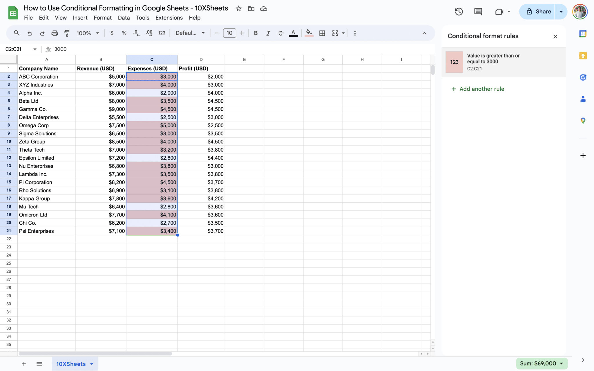
• Setting Conditions: Choose “Single color” or “Color scale” from the formatting styles dropdown, depending on your preference. Then, set the condition based on the cell value. For instance, you could highlight cells greater than a certain value, less than a value, between two values, or equal to a specific value.
  
• Choosing Formatting Options: Select the formatting options you desire, such as text color, background color, or font style. You can also customize the color palette to suit your preferences.
  
• Applying the Formatting: Once you’ve set up the conditions and chosen the formatting options, click “Done” to apply the conditional formatting to the selected range of cells.
  

For example, if you’re analyzing sales data and want to highlight all expenses figures exceeding $3,000, you can set the condition to highlight cells greater than 3000 and choose a bold font style or a different background color to make those values stand out.

Formatting Cells Based on Text Conditions

Conditional formatting is not limited to numeric values; you can also apply it based on specific text conditions. This allows you to highlight cells containing certain keywords or phrases, making it easier to identify relevant information. Here’s how you can do it:

• Selecting the Range: Just like with numeric values, begin by selecting the range of cells containing the text data you want to format conditionally.
• Accessing Conditional Formatting: Navigate to the “Format” menu and select “Conditional formatting.”
• Setting Conditions: Choose “Text contains” from the formatting styles dropdown. Then, enter the text you want to conditionally format for. This can be a single word, a phrase, or even a combination of words.
  
• Choosing Formatting Options: Select the desired formatting options, such as text color, background color, or font style, to apply when the specified text is found.
  
• Applying the Formatting: Click “Done” to apply the conditional formatting to the selected range of cells.
  

For instance, highlight all company names containing Co., Corp, or Corporation, you can set the condition to format cells containing the word “co” with a green background color to make them stand out prominently.

Using Date-Based Conditional Formatting

Dates are a common data type in spreadsheets, and conditional formatting can help you visualize date-related trends or deadlines effectively. Here’s how you can apply date-based conditional formatting:

• Selecting the Range: Select the range of cells containing the date values you want to format conditionally.
• Accessing Conditional Formatting: Go to the “Format” menu and choose “Conditional formatting.”
  
• Setting Conditions: Select “Date is after” or “Date is before” from the formatting styles dropdown, depending on your requirement. Then, specify the date criteria, such as a specific date or a date relative to today.
  
• Choosing Formatting Options: Choose the desired formatting options, such as text color, background color, or font style, to apply when the specified date condition is met.
  
• Applying the Formatting: Click “Done” to apply the conditional formatting to the selected range of cells.
  

For example, if you’re managing project timelines and want to highlight all tasks due after a certain date, you can set the condition to format cells containing dates after the specified deadline with a bold font style or a different background color to signify their urgency.

Advanced Google Sheets Conditional Formatting Techniques

Once you’ve mastered the basics of conditional formatting in Google Sheets, you can explore more advanced techniques to further customize and enhance your spreadsheet visuals. Let’s dive into some advanced methods to apply conditional formatting effectively.

Custom Formula Rules

Custom formula rules offer unparalleled flexibility in conditional formatting, allowing you to create highly specific formatting conditions tailored to your data. With custom formulas, you can apply conditional formatting based on complex logical expressions, mathematical calculations, or even data from other cells.

To create a custom formula rule:

1. Select the Range: Choose the range of cells you want to format conditionally.
2. Access Conditional Formatting: Navigate to the “Format” menu and select “Conditional formatting.”
3. Choose Custom Formula: In the conditional formatting dialog box, select “Custom formula is” from the dropdown menu.
   
4. Enter Formula: Enter your custom formula in the text box provided. This formula should return either TRUE or FALSE for each cell in the selected range, indicating whether the formatting should be applied.
   
5. Define Formatting Options: Specify the formatting options you want to apply when the custom formula evaluates to TRUE.
6. Apply Formatting: Click “Done” to apply the custom formula rule to the selected range of cells.
   

For example, you can create a custom formula to highlight all revenue figures that exceed the average sales value by a certain percentage. For instance, if you want to highlight sales that are 10% higher than the average, you could use a formula like =B2 > AVERAGE(B:B) * 1.10. This formula checks if the revenue figure in cell B2 is greater than 110% of the average sales value in column B. If TRUE, the formatting specified will be applied.

Using Multiple Conditions

In some cases, you may need to apply conditional formatting based on multiple criteria simultaneously. Google Sheets allows you to combine multiple conditions using logical operators (such as AND, OR) to create complex formatting rules.

To apply conditional formatting with multiple conditions:

1. Define Conditions: Identify the multiple criteria you want to apply for conditional formatting, such as highlighting cells that meet two or more specific conditions.
2. Set up Rules: Create separate conditional formatting rules for each condition using the appropriate formatting options.
3. Combine Rules: Use logical operators (AND, OR) to combine the individual rules into a single, comprehensive formatting rule.
   
4. Apply Formatting: Once you’ve defined the combined rule, apply it to the selected range of cells.
   

Let’s say you want to highlight cells where the revenue value in column B is more than $7,000 and the company name in column A contains the text “co”. You can achieve this by using the following custom formula:

=AND(B2 > 7000, SEARCH(“co”, A2) > 0)

This formula checks if the revenue value in cell B2 is greater than $7,000 AND if the company name in cell A2 contains the text “co”. If both conditions are met, the specified formatting will be applied.

Google Sheets Conditional Formatting Based on Another Cell

Conditional formatting based on another cell in Google Sheets allows you to dynamically format cells based on the values or conditions of other cells. This powerful feature enables you to create sophisticated formatting rules that respond to changes in your data dynamically.

To apply conditional formatting based on another cell:

1. Select Range: Choose the range of cells you want to format conditionally.
2. Access Conditional Formatting: Go to the “Format” menu and select “Conditional formatting.”
3. Choose Custom Formula: In the conditional formatting dialog box, select “Custom formula is” from the dropdown menu.
4. Enter Formula: Enter a custom formula that references the cell whose value or condition you want to base the formatting on. For example, if you want to format cells based on whether they are greater than the value in cell A1, you would use a formula like =B1>A1.
5. Define Formatting Options: Specify the formatting options you want to apply when the custom formula evaluates to TRUE.
6. Apply Formatting: Click “Done” to apply the conditional formatting to the selected range of cells.

Suppose you have Expenses in column C and Profit in column D, and you want to highlight the expenses if they’re more than or equal to the profit. You can achieve this by using the following custom formula:

=C2 >= D2

This formula checks if the value in cell C2 (expenses) is greater than or equal to the value in cell D2 (profit). If TRUE, the specified formatting will be applied.

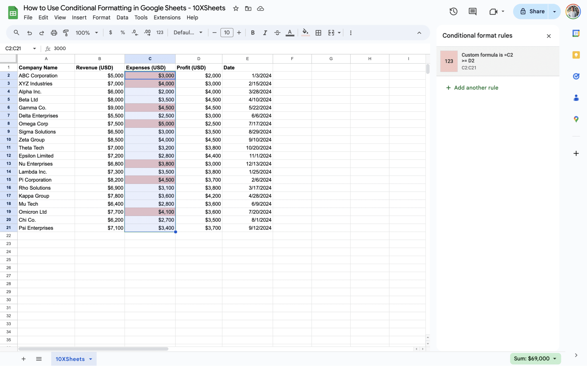
By leveraging conditional formatting based on another cell, you can create dynamic and responsive visualizations that adapt to changes in your data, providing valuable insights at a glance.

Applying Conditional Formatting Across Sheets

Conditional formatting rules can be applied across multiple sheets within the same Google Sheets document, allowing you to maintain consistent formatting throughout your workbook. This is particularly useful when you have related data spread across different sheets and want to ensure uniform visualization.

To apply conditional formatting across sheets:

1. Select Ranges: Identify the ranges of cells you want to format conditionally on each sheet.
2. Define Formatting Rules: Set up the conditional formatting rules for each range of cells, specifying the desired formatting options.
3. Copy Formatting: Once you’ve set up the formatting rules on one sheet, you can easily copy them to other sheets by using the “Copy formatting” option.
4. Paste Formatting: Navigate to the target sheet(s) and paste the copied formatting rules onto the corresponding ranges of cells.

By applying conditional formatting across sheets, you can ensure consistency in data visualization and streamline your workflow when working with multiple sheets within a single document.

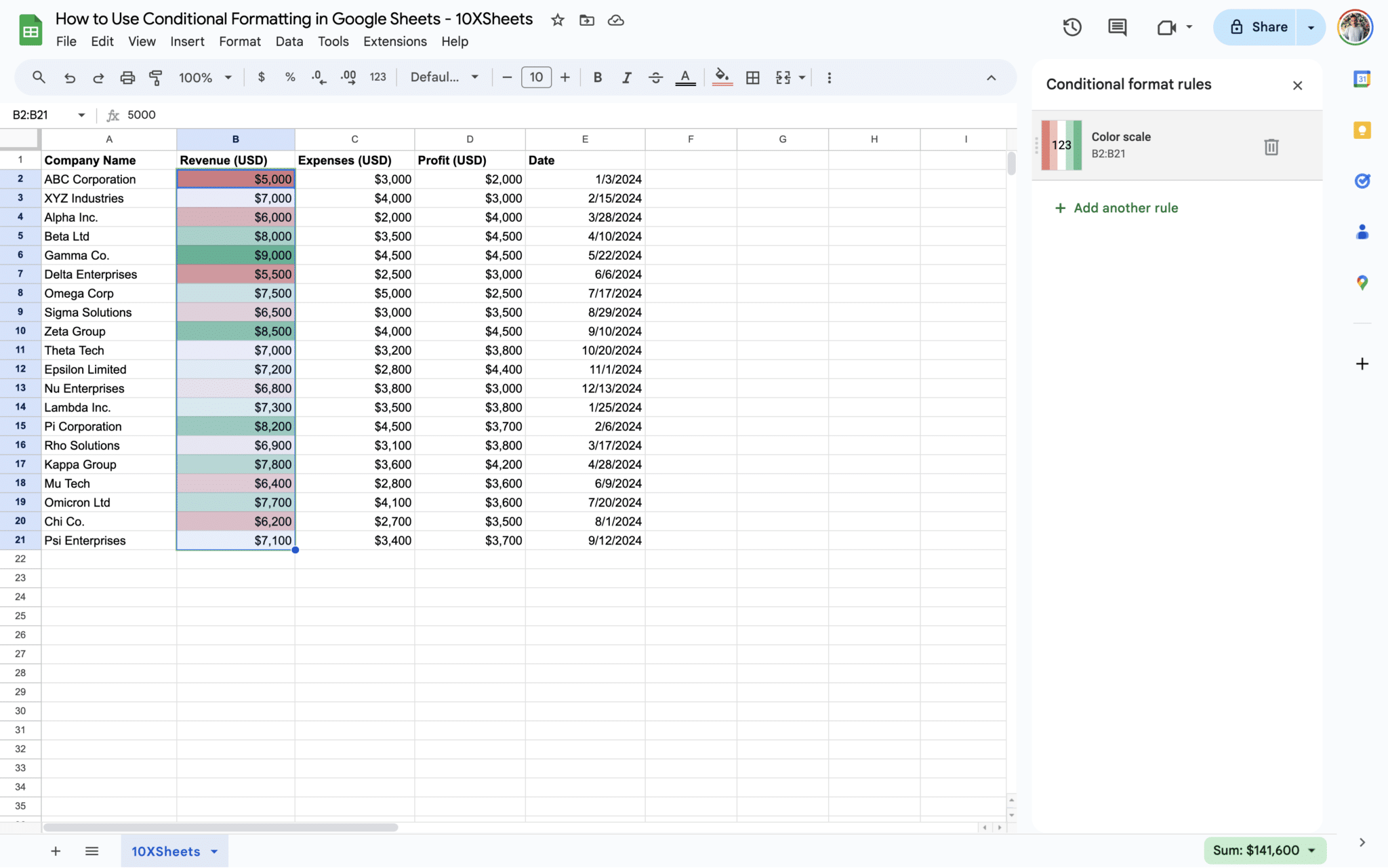
Conditional Formatting with Color Scales and Icon Sets

In addition to single-color formatting, Google Sheets offers built-in color scales and icon sets that allow you to visualize data trends and variations more intuitively. Color scales apply gradient color schemes to cells based on their relative values, while icon sets use icons to represent data categories or ranges.

To apply color scales or icon sets:

1. Select Range: Choose the range of cells you want to format using color scales or icon sets.
2. Access Conditional Formatting: Go to the “Format” menu and select “Conditional formatting.”
3. Choose Style: Select either “Color scale” or “Icon sets” from the formatting styles dropdown, depending on your preference.
   
4. Define Scale or Icon Criteria: Specify the criteria for the color scale or icon set, such as the number of color gradient levels or the range of values for each icon.
   
5. Apply Formatting: Click “Done” to apply the selected color scale or icon set to the range of cells.
   

Color scales and icon sets provide a visually appealing way to represent data variations, making it easier to identify patterns, trends, and outliers within your spreadsheet.

How to Manage Conditional Formatting Rules in Google Sheets?

Now that you’ve applied conditional formatting to your Google Sheets and created various rules to visually enhance your data, it’s essential to know how to manage these rules efficiently. In this section, we’ll explore various management tasks, including editing, deleting, reordering, and copying/pasting formatting rules.

Editing Existing Rules

Editing existing conditional formatting rules allows you to modify the criteria or formatting options to better suit your evolving needs. Here’s how you can edit existing rules:

1. Select Range: Begin by selecting the range of cells containing the conditional formatting rule you want to edit.
2. Access Conditional Formatting: Go to the “Format” menu and select “Conditional formatting.”
3. Modify Rule: In the conditional formatting dialog box, you’ll see a list of existing rules applied to the selected range. Click on the rule you want to edit.
4. Adjust Criteria: Modify the criteria or conditions of the rule as needed. This might involve changing the range of cells, adjusting the formula, or updating the formatting options.
5. Save Changes: Once you’ve made the necessary adjustments, click “Done” to save the edited rule.

By regularly reviewing and updating your conditional formatting rules, you can ensure that they continue to effectively highlight relevant data points and insights within your spreadsheet.

Deleting Conditional Formatting Rules

At times, you may find that certain conditional formatting rules are no longer necessary or relevant. Deleting these rules helps declutter your spreadsheet and streamline your formatting. Here’s how you can delete conditional formatting rules:

1. Select Range: Start by selecting the range of cells containing the conditional formatting rule(s) you want to delete.
2. Access Conditional Formatting: Navigate to the “Format” menu and choose “Conditional formatting.”
3. Identify Rule: In the conditional formatting dialog box, locate the rule you want to delete from the list of existing rules.
4. Delete Rule: Click on the rule to select it, then click the trash can icon or the “Remove rule” option to delete it.
   

Deleting unnecessary formatting rules helps maintain clarity and simplicity in your spreadsheet, ensuring that only relevant formatting is applied to your data.

Reordering Rules

When you have multiple conditional formatting rules applied to the same range of cells, the order in which these rules are evaluated can impact the final formatting outcome. Reordering rules allows you to prioritize certain conditions over others. Here’s how you can reorder conditional formatting rules:

1. Access Conditional Formatting: Start by navigating to the “Format” menu and selecting “Conditional formatting.”
2. Identify Rules: In the conditional formatting dialog box, review the list of existing rules applied to the selected range.
3. Adjust Priority: To change the order of rules, click and drag the rule you want to reorder to the desired position in the list.
4. Save Changes: Once you’re satisfied with the new rule order, click “Done” to save the changes.

By strategically arranging your conditional formatting rules, you can ensure that the most relevant and impactful formatting conditions take precedence, leading to more effective data visualization.

Copying and Pasting Formatting Rules

If you’ve created a formatting rule that you want to apply to a different range of cells or even another sheet within the same document, you can easily copy and paste the formatting rule. Here’s how:

1. Select Range: Begin by selecting the range of cells containing the conditional formatting rule you want to copy.
2. Access Conditional Formatting: Go to the “Format” menu and choose “Conditional formatting.”
3. Copy Formatting: In the conditional formatting dialog box, click on the rule you want to copy to select it. Then, click the three dots menu icon and choose “Copy rule.”
4. Navigate to Target Range: Navigate to the sheet and range of cells where you want to apply the copied formatting rule.
5. Paste Formatting: Select the target range of cells, go to the “Format” menu, choose “Conditional formatting,” and then click the three dots menu icon. Finally, select “Paste special” and choose “Paste conditional formatting only.”

By copying and pasting formatting rules, you can maintain consistency and efficiency in your data visualization across different parts of your spreadsheet.

Google Sheets Conditional Formatting Tips and Best Practices

As you continue to work with conditional formatting in Google Sheets, it’s essential to follow certain tips and best practices to maximize its effectiveness and streamline your workflow. Let’s explore some valuable tips and strategies for optimizing your use of conditional formatting.

Organizing Rules for Efficiency

Efficient organization of conditional formatting rules can greatly enhance your productivity and make it easier to manage your spreadsheet. Consider the following strategies for organizing your rules effectively:

• Group Similar Rules: Organize your conditional formatting rules into logical groups based on their purpose or criteria. For example, you might create separate groups for rules related to sales data, project timelines, or task priorities.
• Use Descriptive Names: Assign descriptive names to your formatting rules that clearly indicate their purpose or conditions. This makes it easier to identify and understand the purpose of each rule, especially when working with a large number of rules.
• Prioritize Rules: Arrange your rules in order of priority, with the most important or frequently used rules at the top of the list. This ensures that critical formatting conditions are applied first, followed by less critical ones.

By organizing your conditional formatting rules thoughtfully, you can streamline your workflow, improve clarity, and make it easier to maintain and update your formatting as needed.

Testing and Previewing Formatting

Before applying conditional formatting to your entire dataset, it’s a good idea to test and preview your formatting rules on a smaller sample. This allows you to ensure that the formatting produces the desired visual effect and does not inadvertently obscure or distort your data. Here’s how you can test and preview your formatting:

• Apply to Sample Data: Select a subset of your data or a test range where you can apply the conditional formatting rules.
• Review Formatting: Apply the formatting rules to the sample data and review the visual impact. Pay attention to how the formatting affects the readability and interpretation of your data.
• Make Adjustments: If necessary, make adjustments to the formatting rules based on your review. This might involve fine-tuning the conditions, tweaking the formatting options, or reordering the rules.
• Confirm Effectiveness: Once you’re satisfied with the formatting applied to the sample data, proceed to apply the same rules to your full dataset.

By testing and previewing your conditional formatting before applying it widely, you can catch any potential issues early on and ensure that your data remains clear and interpretable.

Avoiding Common Pitfalls

While conditional formatting can be a powerful tool for data visualization, it’s important to be aware of common pitfalls that can impact its effectiveness. Here are some common pitfalls to avoid:

• Overcomplicating Rules: Avoid creating overly complex formatting rules that are difficult to understand or maintain. Keep your rules simple and focused on highlighting the most important aspects of your data.
• Conflicting Rules: Be mindful of conflicting formatting rules that may produce unintended or contradictory formatting effects. Review your rules carefully to ensure they work harmoniously together.
• Ignoring Accessibility: Consider the accessibility of your conditional formatting choices, particularly for users with color vision deficiencies or other visual impairments. Use a combination of color, text formatting, and other visual cues to convey information effectively.

By staying vigilant and mindful of these common pitfalls, you can ensure that your conditional formatting enhances the clarity and readability of your data without introducing confusion or errors.

Conclusion

Mastering the art of conditional formatting in Google Sheets opens up a world of possibilities for organizing, analyzing, and presenting your data. By applying formatting rules based on specific conditions, you can transform your spreadsheet into a dynamic visual tool that communicates insights at a glance. Whether you’re highlighting sales trends, tracking project deadlines, or identifying outliers, conditional formatting empowers you to make sense of your data with clarity and efficiency.

Remember, the key to effective conditional formatting lies in understanding your data and defining formatting rules that align with your analysis goals. With practice and experimentation, you’ll become adept at leveraging conditional formatting to uncover valuable insights and make data-driven decisions.